Functions and algebra: Investigate and use instantaneous rate of change of a variable when interpreting models both in mathematical and real life situations
Unit 5: Sketch cubic functions
Natashia Bearam-Edmunds
Unit outcomes
By the end of this unit you will be able to:
- Determine the shape of a cubic function.
- Determine the x and y intercepts.
- Find the turning points of the graph.
- Find the maximum and minimum values of the graph.
- Find the point of inflection and discuss concavity using second derivatives.
What you should know
Before you start this unit, make sure you can:
- Find the derivative by using the rules of differentiation.
- Sketch and interpret information from graphs of functions. Revise level 3 subject outcome 2.1 for a refresher on functions.
Introduction
We have worked with cubic polynomials in this subject outcome. Cubic functions are of the form [latex]\scriptsize y=a{{x}^{3}}+b{{x}^{2}}+cx+d[/latex]. The highest power or degree of a cubic function is three. This also tells us that the graph will have at most three x-intercepts.
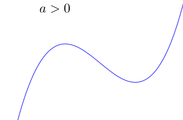
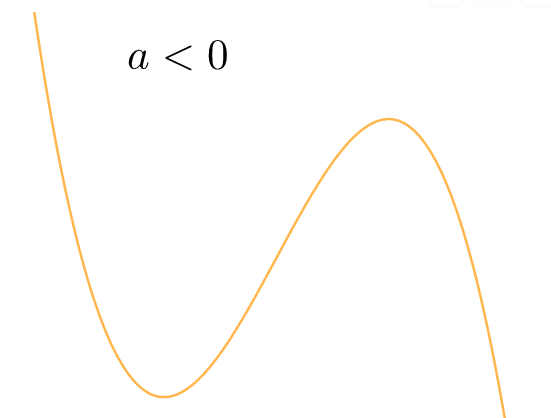
There are two general shapes for cubic functions depending on the value of [latex]\scriptsize a[/latex] the co-efficient of [latex]\scriptsize {{x}^{3}}[/latex].
When [latex]\scriptsize a \gt 0[/latex], the graph starts out concave down (sad [latex]\scriptsize \cap[/latex]) and ends up concave up (happy [latex]\scriptsize \cup[/latex]).
When [latex]\scriptsize a \lt 0[/latex] the graph starts out concave up (happy) and ends up concave down (sad).
Sketching a cubic function
To sketch a cubic function you need the:
- shape
- x- intercepts
- y-intercept
- turning points.
To find the x-intercepts:
- let [latex]\scriptsize \displaystyle y=0[/latex]
- factorise by using the factor theorem
- solve.
To find the y-intercept:
- let [latex]\scriptsize \displaystyle x=0[/latex] and solve for [latex]\scriptsize \displaystyle y[/latex].
Example 5.1
Find the x and y-intercepts of [latex]\scriptsize f(x)=-{{x}^{3}}+4{{x}^{2}}+x-4[/latex].
Solution
To find the y-intercept let [latex]\scriptsize x=0[/latex] and solve for [latex]\scriptsize y[/latex].
[latex]\scriptsize \begin{align*}f(0)&=-{{(0)}^{3}}+4{{(0)}^{2}}+(0)-4\\&=-4\end{align*}[/latex]
The coordinates of the y-intercept are[latex]\scriptsize (0;-4)[/latex].
To find the x-intercepts you will need to use the factor theorem since we must factorise a cubic expression.
[latex]\scriptsize f(x)=-{{x}^{3}}+4{{x}^{2}}+x-4[/latex]
We use trial and error to find factors of [latex]\scriptsize f(x)[/latex]. Remember that a factor will leave no remainder when it divides into an expression.
[latex]\scriptsize \begin{align*}f(1)&=-{{(1)}^{3}}+4{{(1)}^{2}}+(1)-4\\&=0\end{align*}[/latex]
[latex]\scriptsize x=1[/latex] leaves no remainder so one factor of the expression is [latex]\scriptsize (x-1)[/latex].
Factorise further by inspection (or other methods as shown in level 4 subject outcome 2.1).
[latex]\scriptsize \begin{align*}f(x)&=-{{x}^{3}}+4{{x}^{2}}+x-4\\&=-({{x}^{3}}-4{{x}^{2}}-x+4)\\&=-(x-1)({{x}^{2}}-3x-4)\\&=-(x-1)(x-4)(x+1)\end{align*}[/latex]
To find the x-intercepts let [latex]\scriptsize f(x)=0[/latex] and solve for [latex]\scriptsize x[/latex].
[latex]\scriptsize \displaystyle \begin{align*}0&=-(x-1)(x-4)(x+1)\\x&=1,\text{ }x=4\text{ or }x=-1\end{align*}[/latex]
The coordinates of the x-intercepts are [latex]\scriptsize \displaystyle (-1;0),\text{ }(1;0)\text{ and }(4;0)[/latex] .
Exercise 5.1
Determine the x and y-intercepts of the following functions:
- [latex]\scriptsize f(x)=-{{x}^{3}}-5{{x}^{2}}+9x+45[/latex]
- [latex]\scriptsize y={{x}^{3}}+3{{x}^{2}}-10x[/latex]
- [latex]\scriptsize y=2{{x}^{3}}-32x[/latex]
The full solutions are at the end of the unit.
Stationary points
The turning points of a graph are called the stationary points. A cubic graph will have at most two turning points. At the stationary points a tangent drawn to graph will have gradient of zero, therefore the gradient of the graph is zero and the derivative also will be zero. You can think of a stationary point as a point where the function stops increasing or decreasing.
There are three types of stationary points; local maximum (maxima), local minimum (minima) and horizontal points of inflection.
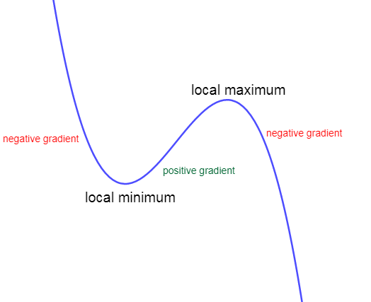
Local maxima or minima are called relative minimum and maximum values, as there are other points on the graph with lower and higher function values.
The gradient of the function changes on either side of local maxima or minima values as shown in figure 3. The function changes from decreasing to increasing at the local minima and changes from increasing to decreasing at the local maxima.
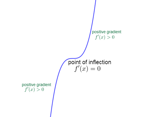
The gradient on either side of a horizontal point of inflection stays constant as shown in figure 4. The graph is increasing on either side of the point of inflection.
To determine the coordinates of the stationary point(s) of [latex]\scriptsize \displaystyle f\left( x \right)[/latex]:
- Find the derivative.
- Let [latex]\scriptsize {f}'(x)=0[/latex] and solve for the x-coordinate(s) of the stationary point(s).
- Substitute value(s) of [latex]\scriptsize \displaystyle x[/latex] into [latex]\scriptsize \displaystyle f\left( x \right)[/latex] to calculate the y-coordinate(s) of the stationary point(s).
Example 5.2
Calculate the stationary point(s) of the graph [latex]\scriptsize f(x)=-{{x}^{3}}+4{{x}^{2}}+3x-4[/latex].
Solution
Step 1: Determine the derivative of [latex]\scriptsize \displaystyle f\left( x \right)[/latex].
[latex]\scriptsize {f}'(x)=-3{{x}^{2}}+8x+3[/latex]
Step 2: Let [latex]\scriptsize \displaystyle {f}'\left( x \right)=0[/latex] and solve for the x-values of the turning point(s).
[latex]\scriptsize \displaystyle \begin{align*}-3{{x}^{2}}+8x+3&=0\\3{{x}^{2}}-8x-3&=0\\(3x+1)(x-3)&=0\\x&=-\displaystyle \frac{1}{3}\text{ and }x=3\end{align*}[/latex]
Step 3: Substitute the x-values into [latex]\scriptsize \displaystyle f\left( x \right)[/latex] to calculate the corresponding y-coordinates of the stationary points.
[latex]\scriptsize \displaystyle \begin{align*}f(-\displaystyle \frac{1}{3})&=-{{(-\displaystyle \frac{1}{3})}^{3}}+4{{(-\displaystyle \frac{1}{3})}^{2}}+3(-\displaystyle \frac{1}{3})-4\\&=-\displaystyle \frac{{122}}{{27}}\\\\f(3)&=-{{(3)}^{3}}+4{{(3)}^{2}}+3(3)-4\\&=14\end{align*}[/latex]
Step 4: Write the final answer.
The stationary points are [latex]\scriptsize \displaystyle (-\displaystyle \frac{1}{3}\text{;-}\displaystyle \frac{{122}}{{27}}\text{) and (3;14)}[/latex].
Exercise 5.2
Find the turning points of the following functions:
- [latex]\scriptsize f(x)=-{{x}^{3}}-3{{x}^{2}}+9x-10[/latex]
- [latex]\scriptsize y={{x}^{3}}+3{{x}^{2}}-10x[/latex]
- [latex]\scriptsize y=2{{x}^{3}}-54x+40[/latex]
The full solutions are at the end of the unit.
Now, we are ready to sketch a cubic function.
General method for sketching cubic graphs:
- Use the sign of [latex]\scriptsize a[/latex] to determine the general shape of the graph.
- Determine the y-intercept by letting [latex]\scriptsize x=0[/latex].
- Determine the x-intercepts by letting [latex]\scriptsize y=0[/latex] and solving for [latex]\scriptsize x[/latex].
- Find the x-coordinates of the turning points by letting [latex]\scriptsize {f}'(x)=0[/latex] and solving for [latex]\scriptsize x[/latex].
- Determine the y-coordinates of the turning points by substituting their x-values into [latex]\scriptsize f(x)[/latex].
- Plot the points and join as a smooth curve.
Example 5.3
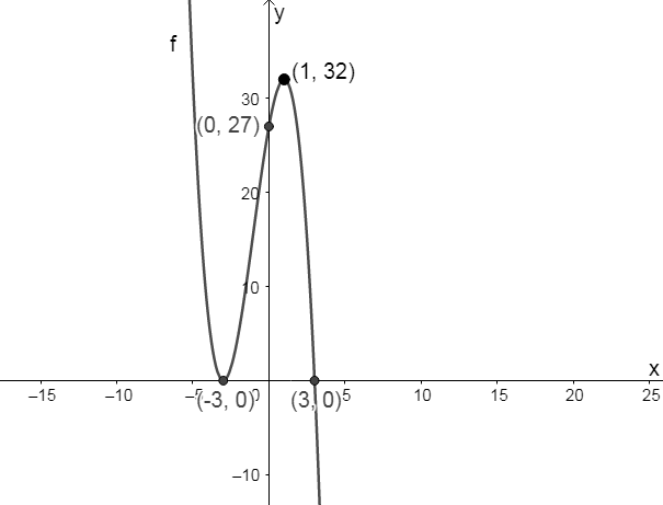
Sketch the graph [latex]\scriptsize f(x)=-{{x}^{3}}-3{{x}^{2}}+9x+27[/latex].
Solution
Step 1: Determine the shape of the graph.
The coefficient of the [latex]\scriptsize {{x}^{3}}[/latex] term is less than zero, therefore the graph will have the following shape:
Step 2: Determine the intercepts.
To find the y-intercept let [latex]\scriptsize x=0[/latex] and solve for [latex]\scriptsize y[/latex].
[latex]\scriptsize \begin{align*}f(0)&=-{{x}^{3}}-3{{x}^{2}}+9x+27\\&=27\end{align*}[/latex]
y-intercept: [latex]\scriptsize (0;27)[/latex]
Find the x-intercepts by letting [latex]\scriptsize f(x)=0[/latex] and solving for [latex]\scriptsize x[/latex]:
[latex]\scriptsize \begin{align*}-{{x}^{3}}-3{{x}^{2}}+9x+27&=0\\{{x}^{3}}+3{{x}^{2}}-9x-27&=0\\(x+3)({{x}^{2}}-9)&=0\\(x+3)(x+3)(x-3)&=0\\x&=-3\text{ or }x=3\end{align*}[/latex]
x-intercepts: [latex]\scriptsize (-3;0)[/latex]and [latex]\scriptsize (3;0)[/latex]
Step 3: Calculate the stationary/turning points.
[latex]\scriptsize \begin{align*}{f}'(x)&=-3{{x}^{2}}-6x+9\\-3{{x}^{2}}-6x+9&=0\\{{x}^{2}}+2x-3&=0\\(x+3)(x-1)&=0\\x&=-3,\text{ }x=1\\f(-3)&=-{{(-3)}^{3}}-3{{(-3)}^{2}}+9(-3)+27\\&=0\\f(1)&=-{{(1)}^{3}}-3{{(1)}^{2}}+9(1)+27\\&=32\end{align*}[/latex]
Turning points: [latex]\scriptsize (-3;0)\text{ }[/latex] and [latex]\scriptsize (1;32)[/latex]
Step 4: Draw a neat sketch (not necessarily drawn to scale).
Show all key points on the graph.
Exercise 5.3
- Given [latex]\scriptsize f(x)={{x}^{3}}+{{x}^{2}}-5x+3[/latex]:
- Show that [latex]\scriptsize (x-1)[/latex] is a factor of [latex]\scriptsize f(x)[/latex] and hence find the x-intercepts.
- Determine the y-intercept and turning points.
- Sketch the graph.
- Sketch the graph of [latex]\scriptsize f(x)=-{{x}^{3}}+4{{x}^{2}}+11x-30[/latex]. Show all the turning points and intercepts with the axes.
The full solutions are at the end of the unit.
Second derivative and concavity
A change in the sign of the second derivative shows that there is a change in the direction of the gradient of the original function. To find the second derivative of a function you take the derivative of the first derivative.
The second derivative tells us about the concavity of a graph. Concavity relates to the rate of change of a function’s derivative. Concavity indicates whether the gradient of a curve is increasing, decreasing or constant.
Take note!
If [latex]\scriptsize {{f}'}'(x) \lt 0[/latex], the graph is concave down and there is a local maximum. Tangent lines drawn to the graph lie above the graph. The gradient of the curve decreases as [latex]\scriptsize x[/latex] increases.
If [latex]\scriptsize {{f}'}'(x) \gt 0[/latex], the graph is concave up and there is a local minimum. Tangent lines lie below the graph. The gradient of the curve increases as [latex]\scriptsize x[/latex] increases.
If [latex]\scriptsize {{f}'}'(x)=0[/latex], the graph may have a point of inflection. If [latex]\scriptsize {{f}'}'(x)[/latex] changes sign from one side of the point of inflection to the other, the concavity changes. For a cubic function, the graph will have a point of inflection when [latex]\scriptsize {{f}'}'(x)=0[/latex].
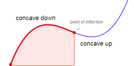
Figure 5 shows how the concavity tells us about the shape of a graph.
Concave down: [latex]\scriptsize {{f}'}'(x) \lt 0[/latex].
Concave up: [latex]\scriptsize {{f}'}'(x) \gt 0[/latex].
Point of inflection: [latex]\scriptsize {{f}'}'(x)=0[/latex] and changes sign at this point.
Exercise 5.4
Determine if the following graphs have a local maximum, minimum or point of inflection at the given points, by finding the second derivative:
- [latex]\scriptsize f(x)=-{{x}^{3}}-3{{x}^{2}}+9x-10[/latex]at [latex]\scriptsize x=1[/latex]
- [latex]\scriptsize y={{x}^{3}}+3{{x}^{2}}-10x[/latex]at [latex]\scriptsize x=-1[/latex]
- [latex]\scriptsize y=2{{x}^{3}}-54x+40[/latex]at [latex]\scriptsize x=3[/latex]
The full solutions are at the end of the unit.
Summary
In this unit you have learnt the following:
- How to identify the shape of a cubic function.
- How to find the x and y-intercepts of a cubic function.
- How to find the stationary points.
- How to find the point of inflection of a cubic function.
- How to test concavity.
- How to sketch a cubic function.
Unit 5: Assessment
Suggested time to complete: 45 minutes
- Given [latex]\scriptsize g(x)={{x}^{3}}-2{{x}^{2}}-3x+6[/latex]:
- Determine the intercepts with the axes.
- Find the stationary points.
- Calculate the point of inflection.
- Sketch the graph.
- Answer the following questions for [latex]\scriptsize f(x)={{(x-2)}^{3}}[/latex]:
- Determine the concavity of the graph.
- Find the inflection point.
- Sketch the graph.
The full solutions are at the end of the unit.
Unit 5: Solutions
Exercise 5.1
- .
[latex]\scriptsize f(x)=-{{x}^{3}}-5{{x}^{2}}+9x+45[/latex]
[latex]\scriptsize \begin{align*}f(3)&=0\\\therefore &(x-3)\text{ is a factor}\end{align*}[/latex]
[latex]\scriptsize \begin{align*}f(x)&=-({{x}^{3}}+5{{x}^{2}}-9x-45)\\&=-(x-3)({{x}^{2}}+8x+15)\\&=-(x-3)(x+3)(x+5)\end{align*}[/latex]
Find the x-intercepts:
[latex]\scriptsize \displaystyle \begin{align*}&-(x-3)(x+3)(x+5)=0\\&\therefore x=3,\text{ }-3\text{ or }-5\\&\text{x-intercepts :}\\&(-5;0),\text{ }(-3;0)\text{ and }(3;0)\text{ }\end{align*}[/latex]
y-intercept: [latex]\scriptsize (0;45)[/latex]. - .
[latex]\scriptsize \begin{align*}y&={{x}^{3}}+3{{x}^{2}}-10x\\&=x({{x}^{2}}+3x-10)\\&=x(x+5)(x-2)\\&\text{x-intercepts}:\\&(0;0),(2;0)\text{ and }(-5;0)\end{align*}[/latex]
y-intercept: [latex]\scriptsize (0;0)[/latex]. - .
[latex]\scriptsize \displaystyle \begin{align*}y&=2{{x}^{3}}-32x\\&=2x({{x}^{2}}-16)\\&=2x(x-4)(x+4)\\&\text{x-intercepts:}\\&(0;0),(-4;0)\text{ and }(4;0)\end{align*}[/latex]
y-intercept: [latex]\scriptsize (0;0)[/latex].
Exercise 5.2
- .
[latex]\scriptsize \begin{align*}{f}'(x)&=-3{{x}^{2}}-6x+9\\-3{{x}^{2}}-6x+9&=0\\{{x}^{2}}+2x-3&=0\\(x+3)(x-1)&=0\\x&=-3,\text{ }x=1\\f(-3)&=-{{(-3)}^{3}}-3{{(-3)}^{2}}+9(-3)-10\\&=-37\\f(1)&=-{{(1)}^{3}}-3{{(1)}^{2}}+9(1)-10\\&=-5\\\text{Turning points: }&(-3;-37)\text{ and }(1;-5)\end{align*}[/latex] - .
[latex]\scriptsize \displaystyle \begin{align*}{y}' &=3{{x}^{2}}+6x-10\\3{{x}^{2}}+6x-10&=0\\x&=\displaystyle \frac{{-b\pm \sqrt{{{{b}^{2}}-4ac}}}}{{2a}}\\&=\displaystyle \frac{{-6\pm \sqrt{{{{{(6)}}^{2}}-4(3)(-10)}}}}{{2(3)}}\\&=\displaystyle \frac{{-3\pm \sqrt{{39}}}}{3}\\x&=\displaystyle \frac{{-3+\sqrt{{39}}}}{3}\text{ or }x=\displaystyle \frac{{-3-\sqrt{{39}}}}{3}\\x&=0.180...\text{ or }x=-3.081...\end{align*}[/latex]
[latex]\scriptsize \begin{align*}f(0.180...)&=-6.04\\f(-3.081...)&=30.04\\\text{Turning points: }&(0.18;-6.04)\text{ and }(-3.08;30.04)\end{align*}[/latex] - .
[latex]\scriptsize \begin{align*}{y}' &=6{{x}^{2}}-54\\{{x}^{2}}-9&=0\\x&=3,\text{ }x=-3\\f(3)&=2{{(3)}^{3}}-54(3)+40\\&=-68\\f(-3)&=2{{(-3)}^{3}}-54(-3)+40\\&=148\\\text{Turning points: }&(3;-68)\text{ and }(-3;148)\end{align*}[/latex]
Exercise 5.3
- [latex]\scriptsize f(x)={{x}^{3}}+{{x}^{2}}-5x+3[/latex]
- .
[latex]\scriptsize \begin{align*}f(1)&={{(1)}^{3}}+{{(1)}^{2}}-5(1)+3\\&=0\\\therefore (x-1)&\text{ is a factor}\end{align*}[/latex]
[latex]\scriptsize \begin{align*}{{x}^{3}}+{{x}^{2}}-5x+3&=(x-1)({{x}^{2}}+2x-3)\\(x-1)({{x}^{2}}+2x-3)&=0\\{{(x-1)}^{2}}(x+3)&=0\\x&=1\text{ or }x=-3\\\text{x-intercepts:}&\text{ }(1;0)\text{ and }(-3;0)\end{align*}[/latex] - [latex]\scriptsize \text{y-intercept }(0;3)[/latex]
[latex]\scriptsize \begin{align*}{f}'(x)&=3{{x}^{2}}+2x-5\\(3x+5)(x-1)&=0\\x&=-\displaystyle \frac{5}{3}\text{ and }x=1\\f(-\displaystyle \frac{5}{3})&=9.48\\f(1)&=0\\\text{Turning points:}&\text{ }(-\displaystyle \frac{5}{3};9.48)\text{ and }(1;0)\end{align*}[/latex] - .
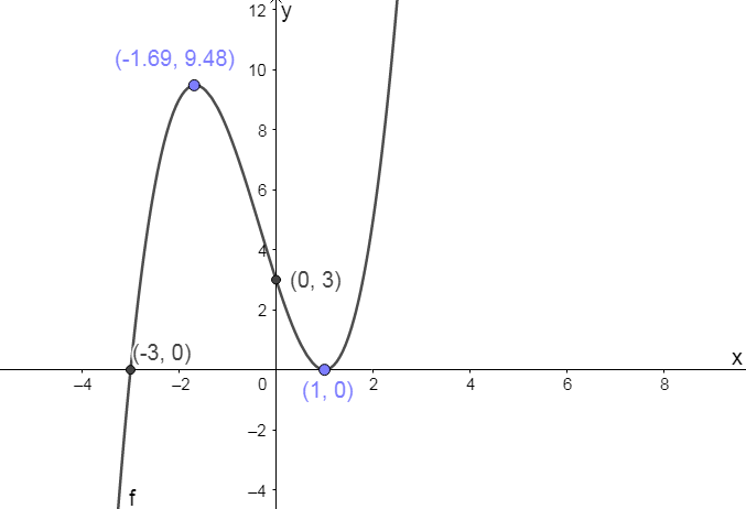
- .
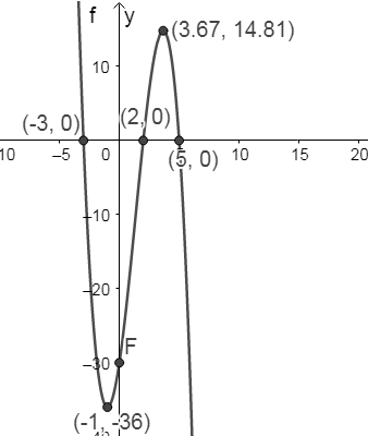
- [latex]\scriptsize f(x)=-{{x}^{3}}+4{{x}^{2}}+11x-30[/latex]

Exercise 5.4
- [latex]\scriptsize {f}'(x)=-3{{x}^{2}}-6x+9[/latex]
[latex]\scriptsize \begin{align*}{{f}'}'(x)&=-6x-6\\{{f}'}'(1)&=-6(1)-6\\&=-12\\{{f}'}'(1)& \lt 0\\\therefore &\text{ local maximum at }x=1\end{align*}[/latex] - [latex]\scriptsize \displaystyle {y}'=3{{x}^{2}}+6x-10[/latex]
[latex]\scriptsize \displaystyle \begin{align*}{{y}'}' &=6x+6\\{{y}'}'(-1)&=0\\\therefore &\text{ there is a point of inflection at }x=-1\\\text{Note:}&\text{ we can make the above statement since y is a cubic function}\text{.}\end{align*}[/latex] - [latex]\scriptsize {y}'=6{{x}^{2}}-54[/latex]
[latex]\scriptsize \begin{align*}{{y}'}' &=12x\\{{y}'}'(3)&=36\\{{y}'}'(3)& \gt 0\\\therefore &\text{ local minimum at }x=3\end{align*}[/latex]
Unit 5: Assessment
- .
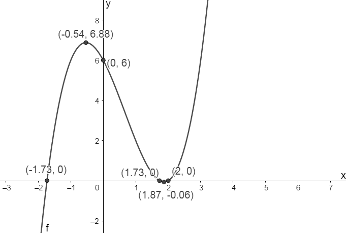
- .
[latex]\scriptsize \begin{align*}g(0)&=6\\\text{y-intercept }(0;6)\\g(2)&=0\\&\therefore (x-2)\text{ is a factor}\\{{x}^{3}}-2{{x}^{2}}-4x+6&=(x-2)({{x}^{2}}-3)\\x&=2\text{ or }x=\pm \sqrt{3}\\\text{x-intercepts:}&\text{ }(2;0),\text{ }(1.73;0)\text{ and }(-1.73;0)\end{align*}[/latex] - .
[latex]\scriptsize \begin{align*}{g}'(x)&=3{{x}^{2}}-4x-3\\3{{x}^{2}}-4x-3&=0 &&\text{ Use the quadratic formula}\\x&=-0.54\text{ or }1.87\\g(-0.54)&=6.88\\g(1.87)&=-0.06\\\text{Stationary points:}&\text{ }(-0.54;6.88)\text{ and }(1.87;-0.06)\end{align*}[/latex] - .
[latex]\scriptsize \begin{align*}{g}'(x)&=3{{x}^{2}}-4x-4\\{{g}'}'(x)&=6x-4\\\text{Note: since }&g\text{ is a cubic function we can let }{g}''(x)=0\text{ to find the point of inflection}\text{.}\\{{g}'}'(x)&=0\\6x-4&=0\\x&=\displaystyle \frac{2}{3}\\\text{Point of inflection:}&\\&(\displaystyle \frac{2}{3};3.41)\end{align*}[/latex] - .
- .
- .
- .
[latex]\scriptsize \displaystyle \begin{align*}{f}'(x)&=3{{(x-2)}^{2}}(1)\\&=3({{x}^{2}}-4x+4)\\&=3{{x}^{2}}-12x+12\\{{f}'}'(x)&=6x-12\\\text{For }x& \lt 2,\text{ the graph is concave down}\text{.}\\\text{For }x& \gt 2,\text{ the graph is concave up}\text{.}\end{align*}[/latex] - .
Note that the function is a cubic:
[latex]\scriptsize \displaystyle \begin{align*}{{f}'}'(x)&=6x-12\\&=0\\\therefore x&=2\\f(2)&=0\\\text{ point of inflection: }&(2;0)\end{align*}[/latex] - .

- .
Media Attributions
- Figure 1 positive cubic © Geogebra is licensed under a CC BY-SA (Attribution ShareAlike) license
- Figure 2 negative cubic © Geogebra is licensed under a CC BY-SA (Attribution ShareAlike) license
- Figure 3 maxima and minima © Geogebra is licensed under a CC BY-SA (Attribution ShareAlike) license
- Figure 4 point of inflection © Geogebra is licensed under a CC BY-SA (Attribution ShareAlike) license
- Figure 6 Example 5.3 © Geogebra is licensed under a CC BY-SA (Attribution ShareAlike) license
- Figure 5 concavity © Geogebra is licensed under a CC BY-SA (Attribution ShareAlike) license
- Exercise 5.3 Q1 © Geogebra is licensed under a CC BY-SA (Attribution ShareAlike) license
- Exercise 5.3 Q2 © Geogebra is licensed under a CC BY-SA (Attribution ShareAlike) license
- Assess Q1 Ans © Geogebra is licensed under a CC BY-SA (Attribution ShareAlike) license
- Assess Q2 Ans © Geogebra is licensed under a CC BY-SA (Attribution ShareAlike) license
