Functions and algebra: Analyse and represent mathematical and contextual situations using integrals and find areas under curves by using integration rules
Unit 1: Introduction to integration
Natashia Bearam-Edmunds
Unit outcomes
By the end of this unit you will be able to:
- Understand the relationship between differentiation and integration (anti-derivative).
- Define integration as the approximate area under curves.
What you should know
Before you start this unit, make sure you can:
- Use the various techniques for differentiation as shown in level 4 subject outcome 2.4.
- Use sigma notation to calculate the sum of a series.
Try these questions to make sure you are ready to start integration.
- Find [latex]\scriptsize \lim_{x \to \infty}\,\displaystyle \frac{2}{x}[/latex]
- Differentiate with respect to [latex]\scriptsize x[/latex]:
- [latex]\scriptsize y=\text{ln2}x[/latex]
- [latex]\scriptsize y=\sin 2x[/latex]
- Calculate [latex]\scriptsize \sum\limits_{{i=1}}^{{12}}{{(4+2i)}}[/latex].
Solutions
- [latex]\scriptsize \lim_{x \to \infty}\,\displaystyle \frac{2}{x}=0[/latex]
- .
- .
[latex]\scriptsize \displaystyle \begin{align*}\displaystyle \frac{d}{{dx}}\ln 2x&=\displaystyle \frac{1}{{2x}}\cdot \displaystyle \frac{d}{{dx}}2x\\&=\displaystyle \frac{1}{{2x}}\cdot 2\\&=\displaystyle \frac{1}{x}\end{align*}[/latex] - .
[latex]\scriptsize \begin{align*}{y}'&=\displaystyle \frac{d}{{dx}}(\sin 2x)\cdot \displaystyle \frac{d}{{dx}}2x\\\displaystyle \frac{d}{{dx}}(\sin 2x)&=\cos 2x\\\displaystyle \frac{d}{{dx}}2x&=2\\\therefore y'&=2\cos 2x\end{align*}[/latex]
- .
- [latex]\scriptsize \sum\limits_{{i=1}}^{{12}}{{(4+2i)}}[/latex]
[latex]\scriptsize \begin{align*}&4+2(1);\text{ }4+2(2);\text{ }4+2(3)...\\&6;8;10...\end{align*}[/latex]
[latex]\scriptsize a=6;\text{ }d=2;\text{ }n=12[/latex]
[latex]\scriptsize \begin{align*}\sum\limits_{{i=1}}^{{12}}{{(4+2i)}}&=\tfrac{{12}}{2}\left( {2(6)+(12-1)2} \right)\\&=6(34)\\&=204\end{align*}[/latex]
Introduction
We live in a world that is in constant motion and changing every instant. It is not static so most ‘real world’ problems need mathematical techniques that can keep up with these instantaneous rates of change. Calculus is the mathematical language that was invented to describe the dynamic nature of our universe.
Calculus is divided into two branches; differential calculus and integral calculus.
In differential calculus you find instantaneous rates of change by dividing something up into infinitely many small slices. In integral calculus, you glue together all these little slices to get back to the bigger picture. The word ‘integration’ means to combine or bring things together. Integration as a mathematical concept has similar meaning.
How do you think integration and differentiation are related?
Mathematically, integration can be thought of in two ways:
- Finding the area under curves.
- Finding the anti-derivative (i.e. undoing differentiation).
In this unit we will discuss both of these approaches to integration.
Estimating areas
Suppose we want to find the area of a circle but do not know the formula. How could we find its area?
One way we could find the area is to place a grid of squares over the circle. Then we can calculate the area of each square and add all of these areas together to estimate the area of the circle. We say it is an estimate of the area because some of the squares will not be completely inside the circle. These squares are highlighted with the blue line in figure 1. Should we count these squares or leave them out?
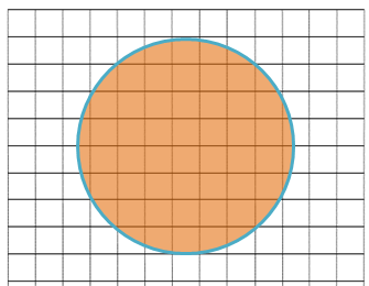
If we add together all the squares that contain any small part of the circle, we will arrive at an overestimate of the area. If we ignore all the squares that do not completely overlap with the circle, then we will underestimate the area.
However, we now have two limits on the area of the circle – an upper one and a lower one. To ‘squeeze’ the area of the circle ever tighter between an upper limit and a lower limit, we would need to make the squares in the grid smaller and smaller. Then the parts that were included or discarded would be, in total, smaller and smaller. The smaller the squares on the grid paper, the better the estimate of the area of the circle. This is called the method of exhaustion.
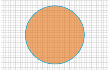
As you can see in figure 2, by dividing a region into many small shapes that have a known area, we can sum these areas and obtain a reasonable estimate of the true area of the circle.
Integration and area under curves
If we know how fast a vehicle is moving, we can use integration to determine how far it travels. Finding distance from velocity is just one of many applications of integration. In fact, integrals are used in a variety of mechanical and physical applications.
In this section, we will learn how to estimate the area under curves. We will come back to the actual calculation of area under curves using integrals in a later unit.
By now you are familiar with finding the area of regular polygons such as squares, rectangles, parallelograms and triangles. Even when these shapes are combined into irregular shapes, it is possible to find the total area by finding the area of the individual shapes and adding those areas together.
For example, you could calculate the area of the ‘tangram man’ in figure 3 by dividing him into several regular shapes as shown in figure 4.


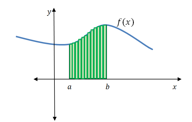
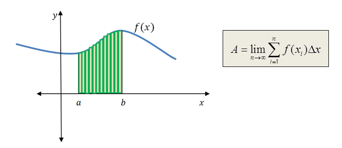
We can extend that idea to find the area bound by the x-axis and any function between two values as seen in figure 5.
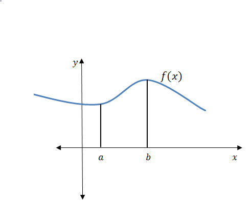
Say we have a function, [latex]\scriptsize f(x)[/latex], and we want to find the area under this curve over a given interval. That means we need to find the area enclosed by the curve [latex]\scriptsize f(x)[/latex], the x-axis and the vertical lines [latex]\scriptsize x=a[/latex] and [latex]\scriptsize x=b[/latex] (a shown in figure 5). Is there a formula we can use to calculate this area?
The curve produces a very irregular shape and the height of the curve is constantly changing as you move between [latex]\scriptsize x=a[/latex] and [latex]\scriptsize x=b[/latex]. Since this shape is not a polygon (a closed shape formed with straight edges) there is no area formula we can use. We need a new technique to find the area under the curve. Integral calculus provides this new technique.
Did you know?
There is a long-standing debate over who invented calculus. It is generally accepted that both Isaac Newton and Gottfried Leibniz invented this revolutionary mathematical idea. For a crash course on the history and development of calculus you can watch this video, Newton and Leibniz: Crash Course History of Science #17.
Think back to how we estimated the area of a circle by adding together the area of all the squares that covered the shape. We can approximate the area of this curved shape in a similar way, using rectangles.
As we did with the circle and squares, we can add rectangles over the area of the curve we want to estimate.

As you can see in figure 6, the big rectangles we have placed do not give the best approximation and over-estimate the area under the curve as they stick out above the curve. But we can make the rectangles ‘narrower’ and place more of them on the diagram. More rectangles mean a better approximation of the area.
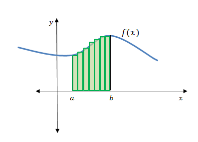
The ‘narrower’ the rectangles, the less they stick out above the curve and the better they approximate with the area under the curve.
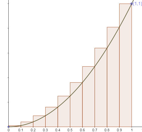
If we take the limit of an infinite number of really narrow rectangles we will be able to get the precise area under the curve. Let us explore this idea quantitatively with the function [latex]\scriptsize f(x)={{x}^{2}}[/latex].
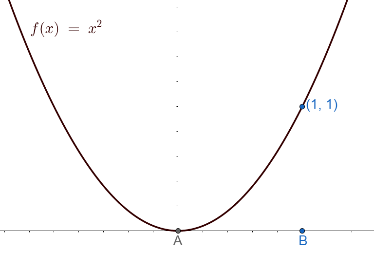
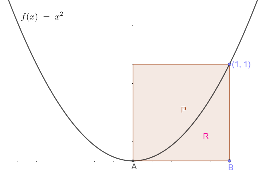
Say we would like to find the area under the curve [latex]\scriptsize f(x)={{x}^{2}}[/latex] between the points [latex]\scriptsize (0;0)[/latex] and [latex]\scriptsize (1,1)[/latex] as shown in figure 10.
We label the area that we are interested in, R. We know that area R will have some value between zero and one. This is because a square, P, in figure 10, with sides of length one unit will have an area of one. Therefore, we can say that [latex]\scriptsize 0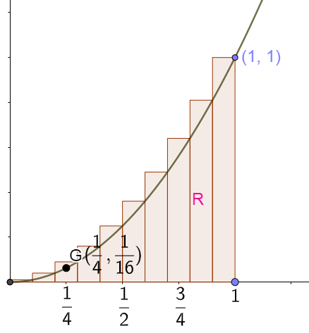 Figure 11: Calculating the area under [latex]\scriptsize f(x)={{x}^{2}}[/latex] using rectangles[/caption]
For example, the point G (in figure 11) will have co-ordinates [latex]\scriptsize (\displaystyle \frac{1}{4},{{(\displaystyle \frac{1}{4})}^{2}})[/latex]. You substitute the x-value into the function to find the y-value. So G is the point[latex]\scriptsize (\displaystyle \frac{1}{4},\displaystyle \frac{1}{{16}})[/latex]. The height of the first rectangle is [latex]\scriptsize \displaystyle \frac{1}{{16}}[/latex] and the width is [latex]\scriptsize \displaystyle \frac{1}{4}[/latex]. Therefore, the first rectangle’s area is [latex]\scriptsize \displaystyle \frac{1}{4}\times \displaystyle \frac{1}{{16}}=\displaystyle \frac{1}{{64}}[/latex]. We continue this way to find the height and area of the remaining three rectangles.
Try finding the areas of each of the other three rectangles yourself.
To find the total area under the curve we add all of the areas together.
| Number of rectangles | Area under the curve |
| [latex]\scriptsize 4[/latex] | [latex]\scriptsize (\displaystyle \frac{1}{4}\times \displaystyle \frac{1}{{16}})+(\displaystyle \frac{1}{4}\times \displaystyle \frac{1}{4})+(\displaystyle \frac{1}{4}\times \displaystyle \frac{9}{{16}})+(\displaystyle \frac{1}{4}\times 1)=0.46875[/latex] |
We know this first approximation is too high because the rectangles stick out above the curve.
Next, we use [latex]\scriptsize 10[/latex] rectangles. These will each have a width of [latex]\scriptsize 0.1[/latex] or [latex]\scriptsize \displaystyle \frac{1}{{10}}[/latex]. This is narrower than the width of the four rectangles used previously. Once again, we can calculate the heights of each rectangle using the function.
| Number of rectangles | Add the area of each rectangle | Approximate area under the curve |
| [latex]\scriptsize 4[/latex] | [latex]\scriptsize (\displaystyle \frac{1}{4}\times \displaystyle \frac{1}{{16}})+(\displaystyle \frac{1}{4}\times \displaystyle \frac{1}{4})+(\displaystyle \frac{1}{4}\times \displaystyle \frac{9}{{16}})+(\displaystyle \frac{1}{4}\times 1)[/latex] | [latex]\scriptsize 0.46875[/latex] |
| [latex]\scriptsize 10[/latex] | [latex]\scriptsize \begin{align*}(0.1\times 0.01)+(0.1\times 0.04)+(0.1\times 0.09)\\+(0.1\times 0.16)+(0.1\times 0.25)+(0.1\times 0.36)\\+(0.1\times 0.49)+(0.1\times 0.64)+(0.1\times 0.81)\\+(0.1\times 1)\end{align*}[/latex] | [latex]\scriptsize 0.385[/latex] |
The rectangles do not stick out as much above the curve so this must be much closer to the actual area but this is still an over-estimate. If we use [latex]\scriptsize 100[/latex] rectangles the rectangles will be much narrower at [latex]\scriptsize 0.01[/latex] units in width. The narrower the rectangles, the closer we will get to the precise area.
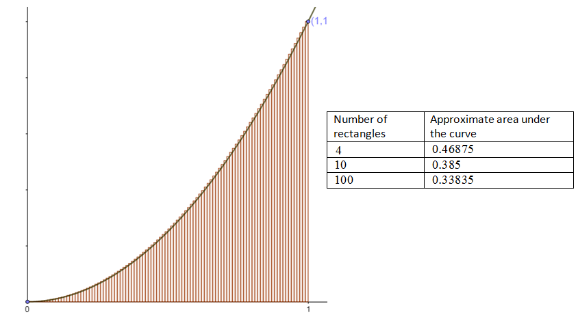
We will not show all of the divisions and calculations, but the table below shows what happens as we increase the number of rectangles all the way to [latex]\scriptsize 1\text{ }000[/latex] rectangles. What number is the area under the curve approaching?
| Number of rectangles | Approximate area under the curve |
| [latex]\scriptsize 4[/latex] | [latex]\scriptsize 0.46875[/latex] |
| [latex]\scriptsize 10[/latex] | [latex]\scriptsize 0.385[/latex] |
| [latex]\scriptsize 100[/latex] | [latex]\scriptsize 0.33835[/latex] |
| [latex]\scriptsize 1000[/latex] | [latex]\scriptsize 0.33383[/latex] |
We can clearly see that area is getting closer and closer to [latex]\scriptsize \displaystyle \frac{1}{3}[/latex]. You will remember from differential calculus that the word we use to indicate ‘getting closer and closer to a specific number’ is, limit.
Actually we can show, and do show in the next unit, that if we take the limit of an infinite number of rectangles, the sum of the areas of the tiny rectangles will be exactly [latex]\scriptsize \displaystyle \frac{1}{3}[/latex]. While we will not show the working here, the area R under the curve [latex]\scriptsize f(x)={{x}^{2}}[/latex] between the points [latex]\scriptsize (0;0)[/latex] and [latex]\scriptsize (1,1)[/latex] is in fact equal to [latex]\scriptsize \displaystyle \frac{1}{3}[/latex].
We can apply this technique to find the area between two values under any function. We can represent the sum of the areas of rectangles using sigma notation.
Take note!
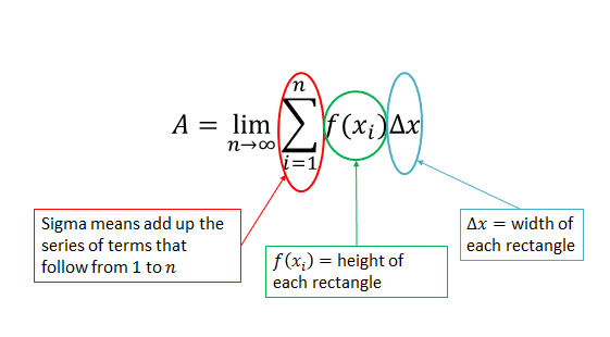
This tells us that we are finding the sum of areas of rectangles.
Taking the [latex]\scriptsize \underset{{n\to \infty }}{\mathop{{\lim }}}\,[/latex] of the sum of an infinite number of rectangles gives the exact area under the curve.
Integration allows us to find the area under a curve. We introduced this idea using sigma notation, but integral notation is much more compact to use when we refer to areas under curves.
Did you know?
Calculus is the foundation of modern science. This animated video explains how integral calculus relates to velocity and time (Duration: 19.03).
[link: https://www.youtube.com/watch?v=rjLJIVoQxz4.]
Integral notation
In differentiation there are special notations and instructional symbols used to indicate the derivative. Similarly, we use special notation and symbols when referring to integrals.
The integral sign [latex]\scriptsize \int{{}}[/latex] which looks like a long ‘s’ is called ‘summa’, the Latin word for sum. When we integrate a function, we use special notation [latex]\scriptsize \int{{f(x)dx}}[/latex]. Each part of integral notation has a name.
Take note!
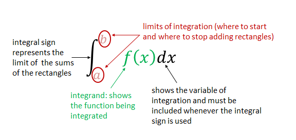 This is called the definite integral and represents the area under a curve for a given interval.
Let us compare sigma notation to integral notation. Which notation would be quicker to write down and easier to work with?
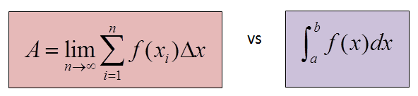
As you can see it is definitely quicker to use integral notation. While both give the area under the curve it is important to note that these notations are only equivalent when we include [latex]\scriptsize n\to \infty[/latex] in the sigma notation, as shown above. For all other values of [latex]\scriptsize n[/latex] the sigma notation only approximates the value of the definite integral. We use [latex]\scriptsize \int_{a}^{b}{{}}[/latex] instead of [latex]\scriptsize \underset{{n\to \infty }}{\mathop{{\lim }}}\,\sum\limits_{{i=1}}^{n}{{}}[/latex] to show that we are calculating the area under a curve.
In the next unit we will show that [latex]\scriptsize \int_{0}^{1}{{{{x}^{2}}dx}}=\displaystyle \frac{1}{3}[/latex]. This is the same as showing that the area under the curve [latex]\scriptsize f(x)={{x}^{2}}[/latex] between the points [latex]\scriptsize (0;0)[/latex] and [latex]\scriptsize (1,1)[/latex] is equal to [latex]\scriptsize \displaystyle \frac{1}{3}[/latex].
Activity 1.1: Explore the area under a curve
Time required: 5 minutes
What you need:
- an internet connection
What to do:
Use the limit of the upper sum of a function to explore the integral.
Click on this link to go to the "Exploring the integral activity".
The following screen should appear:
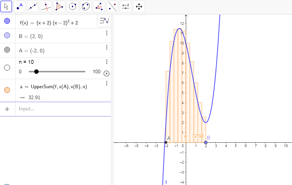
- Press play on the slider [latex]\scriptsize n[/latex] to increase and decrease the number of rectangles over the given interval. Note how the sum of the areas of the rectangles, represented by ‘[latex]\scriptsize a=[/latex]’ on the graph, change. You can change the speed of the rectangles appearing by clicking [latex]\scriptsize \ll[/latex] or [latex]\scriptsize \gg[/latex] above the play button.
- Click the circle next to ‘UpperSum’ to hide the rectangles from the visual. Note: The ‘UpperSum’ gives you the estimate of the area under the curve for different values of [latex]\scriptsize n[/latex] .
- Next, enter the command ‘Integral(f, x(A) ,x(B))’ in the box with the + (input) sign and press enter to display the actual area between [latex]\scriptsize f(x)[/latex] and the x-axis over the given interval. The area will be displayed as ‘[latex]\scriptsize b=[/latex]’ on the graph. This gives the definite integral under the curve over the interval. If you have entered the command correctly it will display a solid shaded region under the curve between A and B. Make sure that the tiny rectangles are hidden or you will not see the area of the definite integral.
- To display the rectangles again, click the circle to the left of ‘UpperSum’. As you change the values of [latex]\scriptsize n[/latex], zoom in on the graph to see how much the rectangles stick out above the curve.
- Drag and hold the points [latex]\scriptsize A[/latex] and [latex]\scriptsize B[/latex] to move the values along the x-axis.
What did you find?
- As [latex]\scriptsize n[/latex] increases to 100 what value does the sum of the areas of the rectangles approach?
- Is the area b displayed using the integral command, Integral(f, x(A) ,x(B)) , close to the sum of the area a of the rectangles as [latex]\scriptsize n\to 100[/latex]?
- Did you get the area of the definite integral [latex]\scriptsize b=29.33[/latex]?

- Did you get the sum of the areas of the tiny rectangles [latex]\scriptsize a=29.71[/latex] when [latex]\scriptsize n=100[/latex]?

The area using summation and the area using the definite integral are close in value ([latex]\scriptsize a=29.71[/latex] and [latex]\scriptsize b=29.33[/latex]). The summation of rectangles helps to approximate the definite integral. As the value of [latex]\scriptsize n[/latex] approaches infinity the area found using the sum of the tiny rectangles will be equal to the area found using the definite integral. - Did you see that the more rectangles you use the less the rectangles stick out above the curve?
Integration reverses differentiation
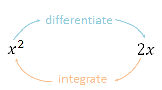
For a known function [latex]\scriptsize f(x)[/latex] we differentiate to find its derivative [latex]\scriptsize {f}'(x)[/latex]. The reverse of this process is to find the original function [latex]\scriptsize F(x)[/latex] from its derivative. In the 17th century the founders of calculus, Isaac Newton and Gottfried Leibniz discovered that integration is the inverse process of differentiation. They proved that evaluating the anti-derivative is equivalent to finding the sum of the areas of an infinite number of rectangles under a curve. So, rather than finding the sum of the areas of an infinite number of tiny rectangles all we have to do to evaluate an integral is invert the process of differentiation.
If we differentiate the function [latex]\scriptsize f(x)={{x}^{2}}[/latex] then its derivative [latex]\scriptsize {f}'(x)=2x[/latex]. So, the integral of [latex]\scriptsize 2x[/latex] takes us back to the original function [latex]\scriptsize {{x}^{2}}[/latex]. We can represent this as shown in figure 15.
Are there other functions that will give us the same derivative of [latex]\scriptsize 2x[/latex]?
There are lots of functions that will have a derivative of [latex]\scriptsize 2x[/latex]. For example, [latex]\scriptsize {{x}^{2}}+2,\text{ }{{x}^{2}}+\displaystyle \frac{1}{4},\text{ }{{x}^{2}}-5[/latex] all have the same derivative [latex]\scriptsize 2x[/latex]. This is because when you differentiate the functions, the derivative of the constant terms will be zero. When we reverse the process of differentiation, we have no idea what the constant term may have been. So we include in the answer a constant of integration, this is an unknown constant, which we call [latex]\scriptsize c[/latex]. Therefore, we say the integral or anti-derivative of [latex]\scriptsize 2x[/latex] is [latex]\scriptsize {{x}^{2}}+c[/latex] and this accounts for all the possible values of the constant term of the function.
Take note!
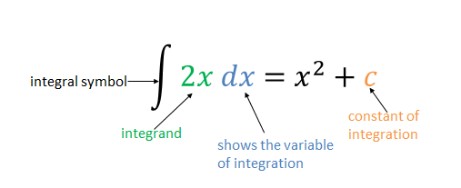
To complete the integral sign there is a term of the form [latex]\scriptsize \displaystyle dx[/latex], which must always be included. It shows the variable involved, in this case [latex]\scriptsize \displaystyle x[/latex]. We read [latex]\scriptsize \int{{2x\text{ }dx}}[/latex] as the integral of [latex]\scriptsize 2x[/latex] with respect to [latex]\scriptsize x[/latex].
The function being integrated is called the integrand. Integrals of this form are called indefinite integrals, to distinguish them from definite integrals, which we will discuss in the next unit.
Indefinite integrals do not have the upper and lower limits of integration as we are finding a function and not the area under a curve. When you find indefinite integrals, your answer must contain a constant of integration.
Take note!
Integration is simply the evaluation of anti-derivatives. This video called "Fundamental theorem of calculus", explains how integration and differentiation are fundamentally linked.
Let’s look at an example to explore this further.
Example 1.1
Find the derivatives of [latex]\scriptsize f(x)={{x}^{3}};\text{ }f(x)={{x}^{3}}+2;\text{ }f(x)={{x}^{3}}-4[/latex]. From there, deduce that [latex]\scriptsize \int 3{{x}^{2}}dx={{x}^{3}}+c[/latex].
Solutions
[latex]\scriptsize f(x)={{x}^{3}}[/latex]and [latex]\scriptsize {f}'(x)=3{{x}^{2}}[/latex]
[latex]\scriptsize f(x)={{x}^{3}}+2[/latex]and [latex]\scriptsize \text{ }{f}'(x)=3{{x}^{2}}[/latex]
[latex]\scriptsize f(x)={{x}^{3}}-4[/latex] and [latex]\scriptsize {f}'(x)=3{{x}^{2}}[/latex]
The derivatives of all three functions are equal.
[latex]\scriptsize \therefore \int{{3{{x}^{2}}dx={{x}^{3}}+c}}[/latex]
Any constant will become zero when differentiated so the constant of integration must be included to cover all possible indefinite integrals.
Rules for integration
There are a number of different rules that are used to make the process of integration simple. In this unit we will focus on the following two rules; the power rule for integrals and the constant coefficient rule.
Power rule for integrals [latex]\scriptsize n\ne -1[/latex]
[latex]\scriptsize \displaystyle \int{{{{x}^{n}}\text{ }dx=\text{ }\displaystyle \frac{{{{x}^{{n+1}}}}}{{n+1}}}}+c[/latex]
Remember from the power rule for differentiation that the derivative of [latex]\scriptsize {{x}^{n}}[/latex] is [latex]\scriptsize n\cdot {{x}^{{n-1}}}[/latex]. To get the anti-derivative we must reverse this process by increasing the exponent by one and then divide the result by the new exponent.
Constant coefficient rule:
[latex]\scriptsize \int{{kf(x)\text{ }dx=k\int{{f(x)\text{ }dx}}}}[/latex]
A constant in an integral can be moved outside the integral sign.
Example 1.2
Find:
- [latex]\scriptsize \displaystyle \int{{\text{4 }dx}}[/latex]
- [latex]\scriptsize \int{{x\text{ }dx}}[/latex]
- [latex]\scriptsize \int{{2{{x}^{2}}\text{ }dx}}[/latex]
Solutions
- .
Here we integrate a constant - the variable has a power of zero.
[latex]\scriptsize \displaystyle \begin{align*}\int{{\text{4 }dx}}=\int{{\text{4}{{x}^{0}}\text{ }dx}}\\=\displaystyle \frac{{4{{x}^{{0+1}}}}}{{0+1}}+c\\=4x+c\end{align*}[/latex] - .
[latex]\scriptsize \displaystyle \begin{align*}\int{{x\text{ }dx}}=\displaystyle \frac{{{{x}^{{1+1}}}}}{{1+1}}+c\\=\displaystyle \frac{{{{x}^{2}}}}{2}+c\end{align*}[/latex]
By using the power rule for integration, we increase the power by one and then divide the result by the new power. - .
[latex]\scriptsize \begin{align*}\int{{2{{x}^{2}}\text{ }dx}}=2\int{{{{x}^{2}}}}\text{ dx}\\\text{=2}\left( {\displaystyle \frac{{{{x}^{{2+1}}}}}{{2+1}}} \right)+c\\=\displaystyle \frac{{2{{x}^{3}}}}{3}+c\end{align*}[/latex]
Keep the constant coefficient.
Note: Since integration is the inverse of differentiation, a way to quickly check your solutions is to derive and see that you arrive at the original expressions.
Exercise 1.1
Find the indefinite integrals of:
- [latex]\scriptsize \int{{5x\text{ }dx}}[/latex]
- [latex]\scriptsize \int{{7\text{ }dt}}[/latex]
- [latex]\scriptsize \int{{{{y}^{3}}\text{ }dy}}[/latex]
- [latex]\scriptsize \int{{\displaystyle \frac{1}{{{{x}^{4}}}}\text{ }dx}}[/latex]
- [latex]\scriptsize \int{{\sqrt{x}\text{ }dx}}[/latex]
The full solutions are at the end of the unit.
Summary
In this unit you have learnt the following:
- How to define the integral as the area under a curve.
- The notation used to represent the definite and indefinite integral.
- The relationship between integration and differentiation.
- How to defined integration as the anti-derivative.
- How to use the power rule for integrals.
- How to use the constant coefficient rule for integrals.
Unit 1: Assessment
Suggested time to complete: 20 minutes
- Use five rectangles to estimate the area under the curve [latex]\scriptsize f(x)={{x}^{2}}[/latex] between the points [latex]\scriptsize (0;0)[/latex] and [latex]\scriptsize (1,1)[/latex] (Hint: the width of each rectangle is [latex]\scriptsize \displaystyle \frac{1}{5}[/latex] ).
- Find the following integrals:
- [latex]\scriptsize \int{{3{{y}^{2}}dy}}[/latex]
- [latex]\scriptsize \int{{\displaystyle \frac{t}{2}}}\text{ }dt[/latex]
- [latex]\scriptsize \int{{\sqrt{{5x}}}}\text{ }dx[/latex]
- [latex]\scriptsize \int{{\sqrt[3]{{8x}}}}\text{ }dx[/latex]
- [latex]\scriptsize \int{{\displaystyle \frac{1}{{\sqrt[4]{t}}}}}\text{ }dt[/latex] Write the answer in root form.
The full solutions are at the end of the unit.
Unit 1: Solutions
Exercise 1.1
- .
[latex]\scriptsize \displaystyle \begin{align*}\int{{5x\text{ }dx}}&=\displaystyle \frac{{5{{x}^{{1+1}}}}}{{1+1}}+c\\&=\displaystyle \frac{{5{{x}^{2}}}}{2}+c\end{align*}[/latex] - .
[latex]\scriptsize \begin{align*}\int{{7\text{ }dt}}&=\displaystyle \frac{{7{{t}^{{0+1}}}}}{{0+1}}+c\\&=7t+c\end{align*}[/latex] Integrate with respect to [latex]\scriptsize t[/latex] - .
[latex]\scriptsize \int{{{{y}^{3}}\text{ }dy}}=\displaystyle \frac{{{{y}^{4}}}}{4}+c[/latex] - .
[latex]\scriptsize \int{{\displaystyle \frac{1}{{{{x}^{4}}}}\text{ }dx}}=\int{{{{x}^{{-4}}}\text{ }dx}}[/latex] Rewrite the integrand using exponents as [latex]\scriptsize {{x}^{{-4}}}[/latex]
[latex]\scriptsize \begin{align*}&=\displaystyle \frac{{{{x}^{{-4+1}}}}}{{-4+1}}+c\\&=-\displaystyle \frac{{{{x}^{{-3}}}}}{3}+c\end{align*}[/latex] - .
[latex]\scriptsize \begin{align*}\int{{\sqrt{x}\text{ }dx}}&=\int{{{{x}^{{\displaystyle \frac{1}{2}}}}\text{ }dx}}\\&=\displaystyle \frac{{{{x}^{{\displaystyle \frac{1}{2}+1}}}}}{{\tfrac{1}{2}+1}}+c\\&=\displaystyle \frac{{{{x}^{{\displaystyle \frac{3}{2}}}}}}{{\tfrac{3}{2}}}+c\\&=\displaystyle \frac{2}{3}\sqrt{{{{x}^{3}}}}+c\end{align*}[/latex]
Unit 1: Assessment
- .
Number of rectangles Coordinates Area under the curve [latex]\scriptsize 5[/latex] [latex]\scriptsize \begin{align*}&(\displaystyle \frac{1}{5},\displaystyle \frac{1}{{25}})\\&(\displaystyle \frac{2}{5},\displaystyle \frac{4}{{25}})\\&(\displaystyle \frac{3}{5},\displaystyle \frac{9}{{25}})\\&(\displaystyle \frac{4}{5},\displaystyle \frac{{16}}{{25}})\\&(1,1)\end{align*}[/latex] [latex]\scriptsize (\displaystyle \frac{1}{5}\times \displaystyle \frac{1}{{25}})+(\displaystyle \frac{1}{5}\times \displaystyle \frac{4}{{25}})+(\displaystyle \frac{1}{5}\times \displaystyle \frac{9}{{25}})+(\displaystyle \frac{1}{5}\times \displaystyle \frac{{16}}{{25}})+(\displaystyle \frac{1}{5}\times 1)=0.44[/latex] - .
- .
[latex]\scriptsize \int{{3{{y}^{2}}dy}}={{y}^{3}}+c[/latex] - .
[latex]\scriptsize \displaystyle \begin{align*}\int{{\displaystyle \frac{t}{2}}}\text{ }dt&=\int{{\displaystyle \frac{1}{2}t}}\text{ }dt\\&=\displaystyle \frac{1}{2}\left( {\displaystyle \frac{{{{t}^{2}}}}{2}} \right)\\&=\displaystyle \frac{{{{t}^{2}}}}{4}+c\end{align*}[/latex] - .
[latex]\scriptsize \begin{align*}\int{{\sqrt{{5x}}}}\text{ }dx&=\int{{\sqrt{5}{{x}^{{\displaystyle \frac{1}{2}}}}}}\text{ }dx\\&=\sqrt{5}\left( {\displaystyle \frac{{{{x}^{{\displaystyle \frac{3}{2}}}}}}{{\tfrac{3}{2}}}} \right)\\&=\displaystyle \frac{{2\sqrt{5}{{x}^{{\displaystyle \frac{3}{2}}}}}}{3}+c\end{align*}[/latex] - .
[latex]\scriptsize \begin{align*}\int{{\sqrt[3]{{8x}}}}\text{ }dx&=\int{{2{{x}^{{\displaystyle \frac{1}{3}}}}}}\text{ }dx\\&=2\left( {\displaystyle \frac{{{{x}^{{\displaystyle \frac{4}{3}}}}}}{{\tfrac{4}{3}}}} \right)\\&=\displaystyle \frac{{3{{x}^{{\displaystyle \frac{4}{3}}}}}}{2}+c\end{align*}[/latex] - .
[latex]\scriptsize \begin{align*}\int{{\displaystyle \frac{1}{{\sqrt[4]{t}}}}}\text{ }dt&=\int{{{{t}^{{\displaystyle \frac{{-1}}{4}}}}}}\text{ }dt\\&=\displaystyle \frac{{{{t}^{{\displaystyle \frac{3}{4}}}}}}{{\tfrac{3}{4}}}\\&=\displaystyle \frac{{4{{t}^{{\displaystyle \frac{3}{4}}}}}}{3}\\&=\displaystyle \frac{4}{3}\sqrt[4]{{{{t}^{3}}}}\end{align*}[/latex]
- .
Media Attributions
- Figure 01 Estimating area of a circle © DHET is licensed under a CC BY (Attribution) license
- Figure 02 Estimating area of a circle_smaller squares © DHET is licensed under a CC BY (Attribution) license
- Figure 03 Tangram man © Public Domain is licensed under a Public Domain license
- Figure 04 Tangram man split into regular shapes © Public Domain is licensed under a Public Domain license
- Area under a curve © DHET is licensed under a CC BY (Attribution) license
- Area under curve big rectangles © DHET is licensed under a CC BY (Attribution) license
- Area under curve narrow rectangles © DHET is licensed under a CC BY (Attribution) license
- Area under curve narrowest rectangles © DHET is licensed under a CC BY (Attribution) license
- Area under parabola on [0;1] © Geogebra is licensed under a CC BY-SA (Attribution ShareAlike) license
- Area R less than area P
- Area under parabola on [0,1] new copy © Geogebra is licensed under a CC BY-SA (Attribution ShareAlike) license
- Area under quadratic 10 rectangles © Geogebra is licensed under a CC BY-SA (Attribution ShareAlike) license
- Area under curve 100 rectangles plus table © Geogebra is licensed under a CC BY-SA (Attribution ShareAlike) license
- Area under curve narrowest rectangles and sigma notation © DHET is licensed under a CC BY (Attribution) license
- Sigma notation explained © DHET is licensed under a CC BY (Attribution) license
- Definite integral introduced © DHET is licensed under a CC BY (Attribution) license
- Sigma notation vs integral notation © DHET is licensed under a CC BY (Attribution) license
- Integral activity image © Geogebra is licensed under a CC BY-SA (Attribution ShareAlike) license
- Integral Activity graph 1 © Geogebra is licensed under a CC BY-SA (Attribution ShareAlike) license
- Integral activity graph 2 © Geogebra is licensed under a CC BY-SA (Attribution ShareAlike) license
- Integral reverse of differentiate © Geogebra is licensed under a CC BY-SA (Attribution ShareAlike) license
- Integral notation © DHET is licensed under a CC BY (Attribution) license

![Area under parabola on [0;1]](https://www.dropbox.com/s/mbj460bgfdp59ic/Area%20under%20parabola%20on%20%5B0%3B1%5D.png?dl=0)
![Area under parabola on [0,1] new copy](https://www.dropbox.com/s/pqw67rmryiv7v6g/Area%20under%20parabola%20on%20%5B0%2C1%5D%20new%20copy.PNG?dl=0)