Data handling: Represent, analyse and interpret data using various techniques
Unit 1: Use various techniques for data collection, representation and interpretation
Natashia Bearam-Edmunds
Unit outcomes
By the end of this unit you will be able to:
- Identify situations or issues that can be dealt with through statistical methods.
- Make resolutions to maximise efficiency from given data which has been organised and graphically represented.
What you should know
Before you start this unit, make sure you can:
- understand basic principles of statistics. You can revise the following statistics units from the previous levels:
Introduction
Social media has a huge impact on the way people interact and the decisions they make. It can also influence many decisions and highlight issues of public importance. A major environmental issue is the need to reduce plastic waste.
This has been widely publicised and the negative effect of plastic on the ocean is well documented. But, what if we wanted to find out how social media reacts to plastic pollution? How could we assess the reaction? To make a conclusion about this question we need to collect information.
The calculation of statistics always starts with collecting information. Why do you think it is important to get information and analyse statistics about plastic waste?
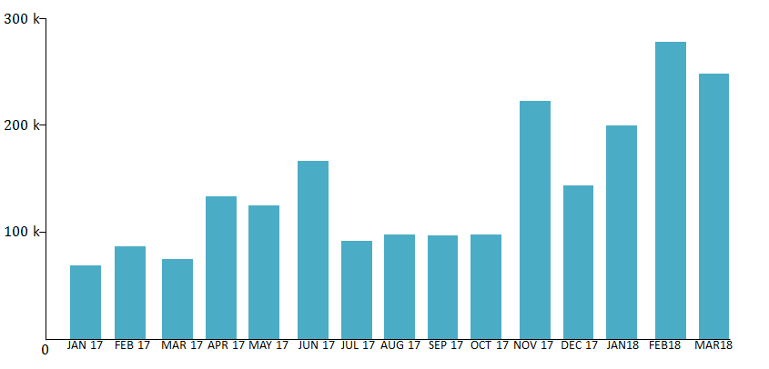
If consumers are becoming more concerned about plastic waste this will influence decisions about the type of products they buy. Businesses need to pay attention to the growing environmental concerns so they can adapt and change their focus to avoid financial pitfalls. In fact, a survey has been done on this very topic. It concluded that people are talking more about the plastics problem on social media, and they are googling the topic more, too. Below is a snapshot of that survey.
From environmental research to sports, statistical calculations are used in almost every field. As you will no doubt encounter statistics somewhere, it is important to be able to analyse statistics and understand how they are computed.
Ask the right questions
To make an informed decision about a current problem, such as plastic pollution, you will need to research the problem and compute statistics. Statistics are calculated for research purposes in many fields. But, not every question justifies the cost and effort of performing statistical research.
Think about situations around you that possibly need further research. So, how do we know if a problem warrants further study? The following will guide your decision to conduct statistical research.
- Can the issue be studied and what is the purpose of the investigation?
- Does it justify further research?
- Is it worth the time, money and effort that will go into the research?
- Is there money available to investigate the issue?
- Are there people with the right skills available to conduct the research?
- Is the size of the sample reasonable to investigate?
- Can you formulate the hypothesis?
A hypothesis is a statement that must be proved or tested through research (observation or experimentation). It is an educated guess and expresses the supposed relationship between two variables. Remember that a variable is something that changes and can have different values or conditions.
For example, if you suspect that time watching TV negatively influences exam results, then your hypothesis could be that the more time you spend watching TV the worse you perform at exams. The variables are time spent watching TV and exam performance.
A hypothesis test involves collecting data from a sample and evaluating the data. Then, a statistician makes a decision whether or not there is sufficient evidence, based on analysis of the data, to reject or accept the hypothesis.
Note
Hypothesis testing is not examinable but it is the basis for most statistical calculations. For your own interest you can learn more about hypothesis testing by watching this video when you have internet access, “Simple hypothesis testing”.
When an issue needs further statistical research we must collect, record, organise and interpret the data using the methods discussed in detail in levels 2 and 3. We will revise those methods next.
Data collection
These are the different types of data that we have worked with so far.
Qualitative data deals with descriptions that can be observed but not measured. For example colours, size, tastes, and appearance.
Categorical data are qualitative. For example hair colour of people at a shopping mall.
Quantitative data deals with numerical data that can be measured. For example length, height, weight, time, cost, and number of people.
Quantitative data are divided into discrete and continuous.
Discrete data are whole number values. For example the number of people attending a maths course.
Continuous data are values that can be measured. For example the heights of learners in an NCV level 4 maths class.
Data sources are varied and include the internet, surveys, censuses and existing records. Often questionnaires, observations and interviews are used to collect data.
In statistics, we generally want to study a population. You can think of a population as a large collection of persons, things, or objects under study. To study the population, we select a sample. The idea of sampling is to select a portion (or subset) of the larger population and study that portion (the sample) to gain information about the population. Data are the result of sampling from a population.
Because it takes a lot of time and money to examine an entire population, sampling is a very practical technique. From the sample data, we can calculate a statistic. A statistic is a number that represents a property of the sample.
The statistic is an estimate of a population parameter. A parameter is a numerical characteristic of the whole population that can be estimated by a statistic.
Data can be collected by sampling in many ways. The simplest way is direct observation.
For example, if you want to find out how many bicycles pass a busy intersection during rush hour traffic, you can stand close to the intersection and count the number of bicycles that pass by in that interval.
Statistics can be a powerful tool in research. Unfortunately, statistics can also have faults. Sample bias is one such fault. Bias is deliberate favouritism when collecting data, resulting in lopsided, misleading results. Bias can occur in the way the sample is chosen and the way the data are collected.
For example, if we wanted to find out how many learners played sport at a college and chose only the male learners to be part of the survey. This will result in misleading results as we have not chosen a sample that is representative of the entire college population, which includes females.
It is important to keep in mind that sampling bias refers to the method of sampling, not the sample itself.
Avoiding bias when selecting a sample
The methods used to collect data must ensure that the data is reliable. This means that it is data that we can trust. Data cannot be trusted unless it has been collected in a way that makes sure that every member of the population under investigation has the same chance of being selected in the sample.
Sample bias occurs when a particular group of the population from which the sample is drawn does not represent that population. The way to avoid sample bias is to take a random sample. A sample is random if every member of the population has an equal chance of being selected.
In addition to the sample being random it must be of an adequate size. The bigger the sample size the more accurate the results.
Example 1.1
Identify the bias in the example below:
Sibusiso collected data from a sample of grade 12 boys at his school to find out how many learners play soccer.
Solution
Since the sample is not random, some individuals are more likely than others to be chosen. Always think very carefully about which individuals are being favoured and how that will influence the results. Sibusiso’s sample is restricted to boys only and is more likely to get a favourable result and skew data. The sample must include girls as well to be a true reflection of the learners at the school.
Organising data
Data is often recorded electronically by using spreadsheets, computer software, scanners and online surveys. The data can then be sorted and organised by:
- grouping using frequency tables
- tallies on tally tables
- stem and leaf diagrams.
Once data are organised it can be summarised so that it can be better analysed.
Summarising data
In levels 2 and 3 we discussed single numerical values that gave us information about the data; measures of central tendency and dispersion. The measures we have already learnt about are the:
- mean
- median
- mode
- range
- lower quartile
- upper quartile
- interquartile range
- semi-interquartile range
- variance and
- standard deviation.
You must be able to calculate the above measures for ungrouped and grouped data, where applicable.
The following formulae are used to calculate the estimated mean, median and mode for grouped data.
Mean:
[latex]\scriptsize \displaystyle \begin{align*}& \bar{x}=\displaystyle \frac{{\sum {{f}_{i}}{{x}_{i}}}}{n}\text{ }\\&{{f}_{i}}{{x}_{i}}\text{ is the class midpoint multiplied by the frequency}\\&n\text{ is the number of observations}\end{align*}[/latex]
Median:
[latex]\scriptsize \displaystyle \begin{align*}&{{\text{M}}_{e}}=l+\displaystyle \frac{{\left( {\displaystyle \frac{n}{2}-F} \right)}}{f}\times c\\&l\text{ is the lower limit of the median class}\\&n\text{ }~\text{is the number of observations}\\&F\text{ is cumulative frequency of the class before the median class}\\&f\text{ is the frequency of the median class}\\&c\text{ is the class width}\end{align*}[/latex]
Mode:
[latex]\scriptsize \begin{align*}&{{M}_{o}}=l+\displaystyle \frac{{{{f}_{m}}-{{f}_{{m-1}}}}}{{2{{f}_{m}}-{{f}_{{m-1}}}-{{f}_{{m+1}}}}}\times c\\&l\text{ is the lower limit of the modal class}\\&{{f}_{m}}\text{ is the frequency of the modal class}\\&{{f}_{{m-1}}}\text{ is the frequency of the class before the modal class}\\&{{f}_{{m+1}}}\text{ is the frequency of the class after the modal class}\\&c\text{ is the class width}\end{align*}[/latex]
Example 1.2
The frequency distribution shows the pulse rates of a group of women.
| Pulse rates of women | Frequency |
| [latex]\scriptsize 60-69[/latex] | [latex]\scriptsize 12[/latex] |
| [latex]\scriptsize 70-79[/latex] | [latex]\scriptsize 14[/latex] |
| [latex]\scriptsize 80-89[/latex] | [latex]\scriptsize 11[/latex] |
| [latex]\scriptsize 90-99[/latex] | [latex]\scriptsize 1[/latex] |
| [latex]\scriptsize 100-109[/latex] | [latex]\scriptsize 1[/latex] |
| [latex]\scriptsize 110-119[/latex] | [latex]\scriptsize 0[/latex] |
| [latex]\scriptsize 120-129[/latex] | [latex]\scriptsize 1[/latex] |
Use the table to find:
- The average pulse rate for the women.
- If these pulse rates are observed in a sample of women admitted to a private hospital is this a good indication of the average pulse rate of all patient admissions?
- Find the median pulse rate.
Solutions
- Find the class midpoints to apply the formula.
Pulse rates of women Class midpoint Frequency [latex]\scriptsize 60-69[/latex] [latex]\scriptsize 64.5[/latex] [latex]\scriptsize 12[/latex] [latex]\scriptsize 70-79[/latex] [latex]\scriptsize 74.5[/latex] [latex]\scriptsize 14[/latex] [latex]\scriptsize 80-89[/latex] [latex]\scriptsize 84.5[/latex] [latex]\scriptsize 11[/latex] [latex]\scriptsize 90-99[/latex] [latex]\scriptsize 94.5[/latex] [latex]\scriptsize 1[/latex] [latex]\scriptsize 100-109[/latex] [latex]\scriptsize 104.5[/latex] [latex]\scriptsize 1[/latex] [latex]\scriptsize 110-119[/latex] [latex]\scriptsize 114.5[/latex] [latex]\scriptsize 0[/latex] [latex]\scriptsize 120-129[/latex] [latex]\scriptsize 124.5[/latex] [latex]\scriptsize 1[/latex] [latex]\scriptsize \displaystyle \begin{align*}\bar{x}&=\displaystyle \frac{{\sum {{f}_{i}}{{x}_{i}}}}{n}\text{ }\\&=\displaystyle \frac{{64.5\times 12+74.5\times 14+84.5\times 11+94.5+104.5+124.5}}{{40}}\\&=\displaystyle \frac{{3\text{ }070}}{{40}}\\&=76.75\end{align*}[/latex]
The average pulse rate for women is [latex]\scriptsize \displaystyle 76.75[/latex]. - No it is not a good representation of the entire population. Male pulse rates are excluded, and the sample size is very small, making this an unreliable sample.
- The median class is [latex]\scriptsize 70-79[/latex].
[latex]\scriptsize \displaystyle \begin{align*}{{\text{M}}_{e}}&=l+\displaystyle \frac{{\left( {\displaystyle \frac{n}{2}-F} \right)}}{f}\times c\\&=70+\displaystyle \frac{{\left( {\displaystyle \frac{{40}}{2}-12} \right)}}{{14}}\times 10\\&=75.71\end{align*}[/latex]
The median pulse rate is [latex]\scriptsize \displaystyle 75.71[/latex].
Example 1.3
On a timed maths test, the lower quartile for time it took to finish the exam was at [latex]\scriptsize \displaystyle 35[/latex] minutes. Interpret the first quartile in the context of this situation.
Solution
This means that [latex]\scriptsize \displaystyle 25\%[/latex] of learners finished the exam in less than [latex]\scriptsize \displaystyle 35[/latex] minutes, or we can say [latex]\scriptsize \displaystyle 75\%[/latex] of learners finished the exam in more than [latex]\scriptsize \displaystyle 35[/latex] minutes.
Representing data
We have used different types of graphs to represent data. Graphs represent data well because they give a picture of the data that is easy to interpret.
Some graphs are better for displaying certain kinds of information than others. The type of graph depends mostly on the type of data that needs to be represented.
| Representation | Advantages |
| Stem-and-leaf diagram | Used to plot data and look at the distribution. All data values within a class are visible. |
| Box-and-whisker diagram | Used to organise data visually. Easy to see the five-number-summary. |
| Bar graph | Used for showing discrete quantitative data or data in categories.
Bar graphs allow us to compare the quantities of different categories, for example, the exam results of different subjects. They are a really good way to show relative sizes. |
| Compound bar graph | Used to compare two or more characteristics for each category. For example, we could use a double-bar graph to compare the differences between male and female preferences for sport to watch. |
| Histogram | Used to represent continuous data that is grouped into equal class intervals, for example height, weight, etc. Histograms are useful to show the way the data is spread out. |
| Pie chart | Used to show a whole divided into parts. They show how the parts relate to each other and how the parts relate to a whole. They do not show the quantities involved. You can use pie charts to show the relative sizes of many things, such as what type of phone people prefer, etc. |
| Broken line graph | Used to show trends or changes in quantities over time, where the categories are related to each other or follow on from each other. For example the categories might be consecutive times, days, months, or years. |
| Ogive (cumulative frequency graph) | Used to determine how many data values lie above or below a particular value in a data set. Ogives are useful for determining the median, percentiles and five number summary of data. |
| Scatter plot | Used to graph data points that have two values associated with them. Data values have two independent measurements, for example, maths marks and science marks. |
You do not need to draw the statistical graphs again in level 4 but you are expected to interpret given graphs and answer questions based on the graphs.
Note
For more information on choosing the correct graph to represent data, you can read about data representations and try examples online.
Example 1.4
The stem-and-leaf diagram shows Drew’s calculus test marks (in percentages) for the year.
| [latex]\scriptsize 3[/latex] | [latex]\scriptsize 5[/latex] |
| [latex]\scriptsize 4[/latex] | [latex]\scriptsize 3[/latex] [latex]\scriptsize 9[/latex] |
| [latex]\scriptsize 5[/latex] | [latex]\scriptsize 8[/latex] [latex]\scriptsize 9[/latex] [latex]\scriptsize 9[/latex] |
| [latex]\scriptsize 6[/latex] | [latex]\scriptsize 5[/latex] [latex]\scriptsize 7[/latex] |
| [latex]\scriptsize 7[/latex] | [latex]\scriptsize 2[/latex] [latex]\scriptsize 5[/latex] [latex]\scriptsize 5[/latex] [latex]\scriptsize 5[/latex] |
| [latex]\scriptsize 8[/latex] | [latex]\scriptsize 1[/latex] [latex]\scriptsize 4[/latex] |
- How many calculus tests did Drew write?
- What is his highest mark?
- What is the modal mark?
- Calculate the mean mark to the nearest percent.
Solution
- Remember: The stem and-leaf diagram is a good choice when the data sets are small. To create the diagram, divide each observation of data into a stem and a leaf. The leaf consists of a final significant digit. For example, [latex]\scriptsize 35[/latex] has stem [latex]\scriptsize 3[/latex] and leaf [latex]\scriptsize 5[/latex]. The decimal [latex]\scriptsize 8.7[/latex] has stem [latex]\scriptsize 8[/latex] and leaf [latex]\scriptsize 7[/latex]. To draw the stem-and-leaf diagram, list the stems vertically from smallest to largest. Draw a vertical line to the right of the stems. Then write the leaves in increasing order next to their corresponding stem.
- There are [latex]\scriptsize 14[/latex] marks listed, so Drew wrote [latex]\scriptsize 14[/latex] tests.
- His highest mark is [latex]\scriptsize 84\%[/latex].
- The modal mark is the one that occurs most often. His modal mark is [latex]\scriptsize 75\%[/latex] as it appears three times.
- Mean mark:
[latex]\scriptsize \begin{align*}\bar{x}&=\displaystyle \frac{{\sum{x}}}{n}\\&=\displaystyle \frac{{35+43+49+58+59+59+65+67+72+3(75)+81+84}}{{14}}\\&=\displaystyle \frac{{897}}{{14}}\\&=64\%\end{align*}[/latex]
Example 1.5
Question adapted from Siyavula Maths Grade 11
The weights of a random sample of boys from a sports club were recorded. The cumulative frequency graph (ogive) below represents the recorded weights.
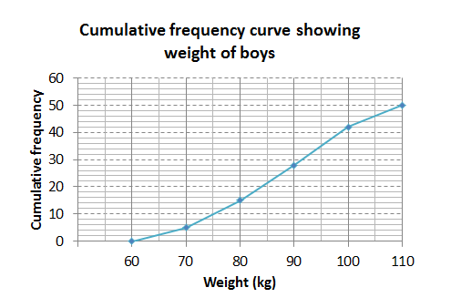
- How many of the boys weighed between [latex]\scriptsize \displaystyle 90[/latex] and [latex]\scriptsize \displaystyle 100[/latex] kilograms?
- Estimate the median weight of the boys.
- If there were [latex]\scriptsize \displaystyle 250[/latex] boys in the club, estimate how many of them would weigh less than [latex]\scriptsize \displaystyle ~80[/latex] kilograms?
- Which other graph(s) could have been used to represent the data?
Solutions
- [latex]\scriptsize 42-28=14[/latex] weighed between [latex]\scriptsize \displaystyle 90[/latex] and [latex]\scriptsize \displaystyle 100[/latex] kilograms.
- Approximately [latex]\scriptsize \displaystyle 88\text{ kg}[/latex].
- [latex]\scriptsize \displaystyle 15[/latex] out of [latex]\scriptsize \displaystyle 50[/latex] boys weigh less than [latex]\scriptsize \displaystyle ~80[/latex] kilograms so [latex]\scriptsize 75[/latex] boys [latex]\scriptsize \left( {\displaystyle \frac{{15}}{{50}}\times 250=75} \right)[/latex] out of the total of [latex]\scriptsize \displaystyle 250[/latex] would weigh less than [latex]\scriptsize \displaystyle ~80[/latex] kilograms.
- A histogram would be an appropriate way to represent the data.
Example 1.6
A group of learners count the number of sweets they each have. This is a histogram describing the data they collected.
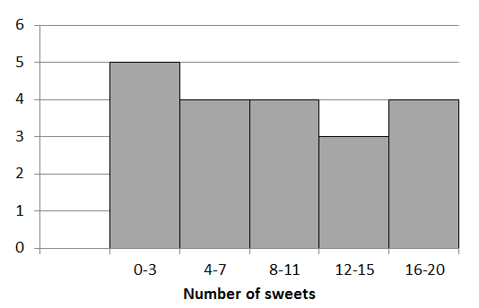
A cat jumps onto the table and all their notes land on the floor, mixed up, by accident! Help them find which of the following data sets match the above histogram:
Data set A
| [latex]\scriptsize 2[/latex] | [latex]\scriptsize 1[/latex] | [latex]\scriptsize 20[/latex] | [latex]\scriptsize 10[/latex] | [latex]\scriptsize 5[/latex] | [latex]\scriptsize 3[/latex] | [latex]\scriptsize 10[/latex] | [latex]\scriptsize 2[/latex] | [latex]\scriptsize 6[/latex] | [latex]\scriptsize 1[/latex] |
| [latex]\scriptsize 2[/latex] | [latex]\scriptsize 2[/latex] | [latex]\scriptsize 17[/latex] | [latex]\scriptsize 3[/latex] | [latex]\scriptsize 18[/latex] | [latex]\scriptsize 3[/latex] | [latex]\scriptsize 7[/latex] | [latex]\scriptsize 10[/latex] | [latex]\scriptsize 8[/latex] | [latex]\scriptsize 18[/latex] |
Data set B
| [latex]\scriptsize 2[/latex] | [latex]\scriptsize 9[/latex] | [latex]\scriptsize 12[/latex] | [latex]\scriptsize 10[/latex] | [latex]\scriptsize 5[/latex] | [latex]\scriptsize 9[/latex] | [latex]\scriptsize 10[/latex] |
| [latex]\scriptsize 13[/latex] | [latex]\scriptsize 6[/latex] | [latex]\scriptsize 5[/latex] | [latex]\scriptsize 11[/latex] | [latex]\scriptsize 10[/latex] | [latex]\scriptsize 7[/latex] | [latex]\scriptsize 2[/latex] |
Data set C
| [latex]\scriptsize 3[/latex] | [latex]\scriptsize 12[/latex] | [latex]\scriptsize 16[/latex] | [latex]\scriptsize 10[/latex] | [latex]\scriptsize 15[/latex] | [latex]\scriptsize 17[/latex] | [latex]\scriptsize 18[/latex] | [latex]\scriptsize 2[/latex] | [latex]\scriptsize 3[/latex] | [latex]\scriptsize 7[/latex] |
| [latex]\scriptsize 11[/latex] | [latex]\scriptsize 12[/latex] | [latex]\scriptsize 8[/latex] | [latex]\scriptsize 2[/latex] | [latex]\scriptsize 7[/latex] | [latex]\scriptsize 17[/latex] | [latex]\scriptsize 3[/latex] | [latex]\scriptsize 11[/latex] | [latex]\scriptsize 4[/latex] | [latex]\scriptsize 4[/latex] |
Solution
Count the number of values in each range of the drawn histogram and compare that to the given tables of data.
Data set A has eight values in the [latex]\scriptsize 0-3[/latex] range but the histogram has five values in that range so A does not match the histogram.
Data set B has one value in the [latex]\scriptsize 0-3[/latex] range so it is not the right match for the histogram.
Data set C has five values in the [latex]\scriptsize 0-3[/latex] range and the number of values in each of the other ranges matches too. Therefore, data set C matches the given histogram.
Note
To learn more about statistical studies watch the video “Types of statistical studies” when you have access to the internet.
Exercise 1.1
- The box-and-whisker diagrams (plots) show the maths test results in percentages for two tests that learners wrote.
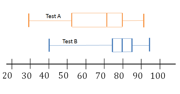
- What is the highest mark in test A?
- What is the lowest mark in test B?
- What is the median mark in test B?
- Between what values do [latex]\scriptsize 50\%[/latex] of the marks lie in test A?
- What mark did [latex]\scriptsize 25\%[/latex] of learners get less than in test B?
- What mark did [latex]\scriptsize 75\%[/latex]of learners get more than in test A?
- Which other graph(s) could have been used to represent the data?
- The cumulative frequency curve shows the percentage improvement in marks of a group of learners after they attended a maths camp.
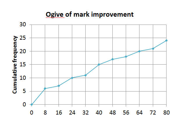
- How many learners attended the maths camp?
- How many learner’ marks improved by [latex]\scriptsize 24[/latex] to [latex]\scriptsize 40\%[/latex]?
- How many learners’ marks increased by [latex]\scriptsize 64\%[/latex] or more?
- Would a box-and-whisker diagram be an appropriate representation for the type of information we are looking for in this case?
The full solutions are at the end of the unit.
Summary
In this unit you have learnt the following:
- How to test if issues warrant further scientific research.
- How to identify graphs that best represent a given data set.
- How to compare different data representations.
Unit 1: Assessment
Suggested time to complete: 20 minutes
- The following ogive shows the test results, in percentages, for a class.
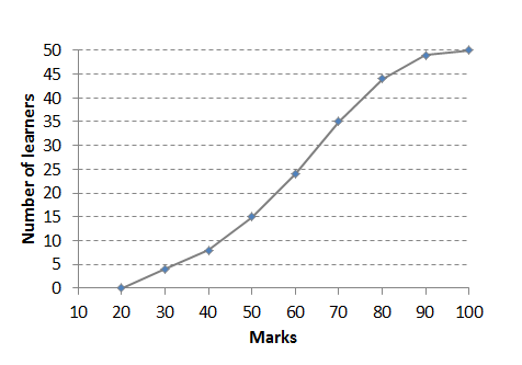
- How many learners are in the class?
- How many learners got [latex]\scriptsize 70\%[/latex] or less?
- [latex]\scriptsize 30\%[/latex]of learners got less than what mark?
- If the pass mark is [latex]\scriptsize 50\%[/latex], how many learners passed?
- What other graph(s) could have been used to represent the data?
- The box-and-whisker plot shows the ages of members at a sports club.
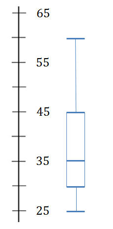
- How old is the youngest member?
- What is the median age?
- Between what ages do the middle [latex]\scriptsize 50\%[/latex] of data values lie?
- Below what age do [latex]\scriptsize 100\%[/latex] of data values lie?
- [latex]\scriptsize 75\%[/latex] of the club membership is older than what age?
- What other graph(s) could have been used to represent the data?
The full solutions are at the end of the unit.
Unit 1: Solutions
Exercise 1.1
- .
- The highest mark in test A is [latex]\scriptsize 90\%[/latex].
- The lowest mark in test B is [latex]\scriptsize 40\%[/latex].
- The median mark in test B is [latex]\scriptsize 80\%[/latex].
- In test A [latex]\scriptsize 50\%[/latex] of the marks lie between [latex]\scriptsize 70\%[/latex] and [latex]\scriptsize 90\%[/latex] (or between [latex]\scriptsize 30\%[/latex] and [latex]\scriptsize 70\%[/latex]).
- [latex]\scriptsize 25\%[/latex] of learners got less than [latex]\scriptsize 75\%[/latex] in test B.
- [latex]\scriptsize 75\%[/latex]of learners got more than [latex]\scriptsize 50\%[/latex] in test A.
- Ogives or compound bar graphs could have been used to represent and compare the data.
- .
- [latex]\scriptsize 24[/latex]
- [latex]\scriptsize 15-10=5[/latex]
- [latex]\scriptsize 4[/latex]
- No a box-and-whisker diagram would not be an adequate representation in this case. The ogive is also known as the ‘less than’ graph and we can easily see what percentages/values are below or above a certain point.
Unit 1: Assessment
- .
- [latex]\scriptsize \displaystyle 50[/latex]
- [latex]\scriptsize \displaystyle 35[/latex]
- [latex]\scriptsize 50\%[/latex]
- [latex]\scriptsize \displaystyle 35[/latex] learners passed.
- A box-and-whisker diagram or bar graph could have been used.
- .
- The youngest member is [latex]\scriptsize 25[/latex] years old.
- [latex]\scriptsize \displaystyle 35[/latex] is the median age.
- The middle [latex]\scriptsize 50\%[/latex] of data values lie between [latex]\scriptsize 30[/latex] and [latex]\scriptsize 45[/latex].
- [latex]\scriptsize 60[/latex]
- [latex]\scriptsize 75\%[/latex] of the club membership is older than [latex]\scriptsize 30[/latex].
- A bar graph or ogive could have been used.
Media Attributions
- Fig 1 Tweets about plastic waste
- Fig 2 Example 1.5 © DHET is licensed under a CC BY (Attribution) license
- Fig 3 Example 1.6 © DHET is licensed under a CC BY (Attribution) license
- Fig 4 Exercise 1.1 Q1 © DHET is licensed under a CC BY (Attribution) license
- Fig 5 Exercise 1.1 Q2 © DHET is licensed under a CC BY (Attribution) license
- Fig 6 Assess Q1 © DHET is licensed under a CC BY (Attribution) license
- Fig 7 Assess Q2 © DHET is licensed under a CC BY (Attribution) license
