Functions and algebra: Analyse and represent mathematical and contextual situations using integrals and find areas under curves by using integration rules
Unit 2: Rules for integration
Natashia Bearam-Edmunds
Unit outcomes
By the end of this unit you will be able to:
- Apply the rules of integration to various functions.
- Calculate the definite integral.
What you should know
Before you start this unit, make sure you can:
- Define integration. To revise this, refer to unit 1 of this subject outcome.
- Apply the various techniques of differentiation by rule. To revise this, refer back to level 4 subject outcome 2.4 unit 1.
- Evaluate simple integrals by reversing the process of differentiation.
Try the following questions to make sure you are ready for this unit.
Find the indefinite integrals of:
- [latex]\scriptsize \int{{5x\text{ }dx}}[/latex]
- [latex]\scriptsize \int{{\sqrt{x}\text{ }dx}}[/latex]
- [latex]\scriptsize \int{{\sqrt[3]{{8x}}}}\text{ }dx[/latex]
Solutions
- .
[latex]\scriptsize \displaystyle \begin{align*}\int{{5x\text{ }dx}}&=\displaystyle \frac{{5{{x}^{{1+1}}}}}{{1+1}}+c\\&=\displaystyle \frac{{5{{x}^{2}}}}{2}+c\end{align*}[/latex] - .
[latex]\scriptsize \begin{align*}\int{{\sqrt{x}\text{ }dx}}&=\int{{{{x}^{{\displaystyle \frac{1}{2}}}}\text{ }dx}}\\&=\displaystyle \frac{{{{x}^{{\displaystyle \frac{1}{2}+1}}}}}{{\tfrac{1}{2}+1}}+c\\&=\displaystyle \frac{{{{x}^{{\displaystyle \frac{3}{2}}}}}}{{\tfrac{3}{2}}}+c\\&=\displaystyle \frac{2}{3}\sqrt{{{{x}^{3}}}}+c\end{align*}[/latex] - .
[latex]\scriptsize \begin{align*}\int{{\sqrt[3]{{8x}}}}\text{ }dx&=\int{{2{{x}^{{\displaystyle \frac{1}{3}}}}}}\text{ }dx\\&=2\left( {\displaystyle \frac{{{{x}^{{\displaystyle \frac{4}{3}}}}}}{{\tfrac{4}{3}}}} \right)\\&=\displaystyle \frac{{3{{x}^{{\displaystyle \frac{4}{3}}}}}}{2}+c\end{align*}[/latex]
Introduction
Integration and differentiation are inverse processes. The inverse relationship between differentiation and integration means that, for every statement about differentiation, there is a corresponding statement about integration. Finding the antiderivative is the same as finding an indefinite integral. The answer to an indefinite integral will always be some function.
Take note!
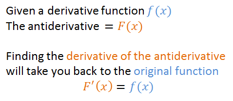
If [latex]\scriptsize \displaystyle \frac{d}{{dx}}\left( {F(x)} \right)=f(x)[/latex] then [latex]\scriptsize \int{{f(x)dx=F(x)}}[/latex].
In other words, if the derivative of [latex]\scriptsize F(x)[/latex] is [latex]\scriptsize f(x)[/latex] , then an indefinite integral of [latex]\scriptsize f(x)[/latex] with respect to [latex]\scriptsize x[/latex] is [latex]\scriptsize F(x)[/latex].
Note: we say an indefinite integral, not the indefinite integral. This is because an indefinite integral is not unique.
In unit 1 you learnt how to apply the power and constant coefficient rules for integration. These rules were fairly straightforward but there are many other integration rules, which get more complicated the more complex the functions become. In this unit we will go over the strategies that you will use when integrating different types of functions.
Integral rules
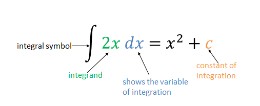
You have already seen, in the previous unit, that there are lots of functions with the same derivative. For example, [latex]\scriptsize {{x}^{2}}+2,\text{ }{{x}^{2}}+\displaystyle \frac{1}{4},\text{ }{{x}^{2}}-5[/latex] all have the same derivative [latex]\scriptsize 2x[/latex]. This is because when you differentiate the functions, the derivative of the constant terms will be zero. When we reverse the process of differentiation, we have no idea what the constant term may have been. So, we include in the answer a constant of integration. This is an unknown constant, which we call [latex]\scriptsize c[/latex].Therefore, we say the indefinite integral or antiderivative of [latex]\scriptsize 2x[/latex] is [latex]\scriptsize {{x}^{2}}+c[/latex] and this accounts for all the possible values of the constant term of the function.
We have defined integration as the inverse of differentiation but more precisely it is an indefinite integral that is the inverse of differentiation.
Take note!
The above integral is called an indefinite integral. Given a function [latex]\scriptsize f(x)[/latex], an indefinite integral of ‘[latex]\scriptsize f[/latex]’ is its most general antiderivative. If [latex]\scriptsize F(x)[/latex] is an antiderivative of ‘[latex]\scriptsize f[/latex]’ then [latex]\scriptsize \displaystyle \int{{f(x)dx=F(x)+c}}[/latex]. The act of finding the antiderivatives of a function is referred to as integrating.
The rules for integration of functions are derived from the rules for differentiation.
Sum and difference rule:
[latex]\scriptsize \int{{(f(x)\pm g(x))dx=\int{{f(x)dx\pm \int{{g(x)dx}}}}}}[/latex]
It sometimes helps to understand and remember rules like this if you state it in words. The above rule states that the integral of the sum (or difference) of two functions is the sum (or difference) of their integrals. We can easily extend this rule to include more than two terms.
For example, [latex]\scriptsize \int{{(5{{x}^{3}}-7{{x}^{2}}+3x+4)dx=\int{{5{{x}^{3}}dx-\int{{7{{x}^{2}}dx}}+\int{{3xdx+\int{{4dx}}}}}}}}[/latex] .
Take note!
You have already applied the following rules in the previous unit.
Power rule for integrals [latex]\scriptsize n\ne -1[/latex]:
[latex]\scriptsize \displaystyle \int{{{{x}^{n}}\text{ }dx=\text{ }\displaystyle \frac{{{{x}^{{n+1}}}}}{{n+1}}}}+c[/latex]
Constant coefficient rule:
[latex]\scriptsize \int{{kf(x)\text{ }dx=k\int{{f(x)\text{ }dx}}}}[/latex]
Example 2.1
Find the following indefinite integrals:
- [latex]\scriptsize \int{{(5{{x}^{3}}-7{{x}^{2}}+3x+4)dx}}[/latex]
- [latex]\scriptsize \int{{\displaystyle \frac{{{{x}^{2}}+4\sqrt[3]{x}}}{x}}}dx[/latex]
Solutions
- Using properties of indefinite integrals, we can integrate each of the four terms in the integrand separately.
[latex]\scriptsize \int{{(5{{x}^{3}}-7{{x}^{2}}+3x+4)dx=\int{{5{{x}^{3}}dx-\int{{7{{x}^{2}}dx}}+\int{{3xdx+\int{{4dx}}}}}}}}[/latex]
From the constant coefficient rule each coefficient can be written in front of the integral sign.
[latex]\scriptsize \int{{5{{x}^{3}}dx-\int{{7{{x}^{2}}dx}}+\int{{3xdx+\int{{4dx}}}}}}=5\int{{{{x}^{3}}dx-7\int{{{{x}^{2}}dx}}+3\int{{xdx+4\int{{1dx}}}}}}[/latex]
Using the power rule for integrals, we get:
[latex]\scriptsize 5\int{{{{x}^{3}}dx-7\int{{{{x}^{2}}dx}}+3\int{{xdx+4\int{{1dx}}}}}}=\displaystyle \frac{5}{4}{{x}^{4}}-\displaystyle \frac{7}{3}{{x}^{3}}+\displaystyle \frac{3}{2}{{x}^{2}}+4x+c[/latex]
Note: We do not repeat the ‘c’ for each term, we use one ‘c’ for the entire integral. - Rewrite the integrand to simplify the exponents.
[latex]\scriptsize \int{{\displaystyle \frac{{{{x}^{2}}+4\sqrt[3]{x}}}{x}}}dx=\int{{\displaystyle \frac{{{{x}^{2}}}}{x}}}+\displaystyle \frac{{4\sqrt[3]{x}}}{x}dx[/latex]
Then, to evaluate the integral, integrate each of these terms separately.
[latex]\scriptsize \displaystyle \begin{align*}\int{{\displaystyle \frac{{{{x}^{2}}}}{x}}}+\displaystyle \frac{{4\sqrt[3]{x}}}{x}dx&=\int{{\displaystyle \frac{{{{x}^{2}}}}{x}}}dx+\int{{\displaystyle \frac{{4{{x}^{{\displaystyle \frac{1}{3}}}}}}{x}}}dx\\&=\int{{xdx+}}\int{{4{{x}^{{\displaystyle \frac{{-2}}{3}}}}dx}}\\&=\displaystyle \frac{1}{2}{{x}^{2}}+4\left( {\displaystyle \frac{{{{x}^{{\displaystyle \frac{{-2}}{3}+1}}}}}{{\tfrac{{-2}}{3}+1}}} \right)+c\\&=\displaystyle \frac{1}{2}{{x}^{2}}+12{{x}^{{\displaystyle \frac{1}{3}}}}+c\end{align*}[/latex]
Exercise 2.1
Find the following integrals using the rules for integration:
- [latex]\scriptsize \int{{(2{{x}^{3}}+{{x}^{2}}-2x)dx}}[/latex]
- [latex]\scriptsize \int{{y(\displaystyle \frac{1}{y}+{{y}^{2}})dy}}[/latex]
- [latex]\scriptsize \int{{(\sqrt{x}+}}\sqrt{{3x}})dx[/latex]
The full solutions are at the end of the unit.
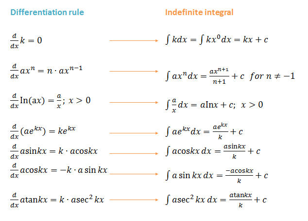
Differentiation rules make integrating simple
The key to understanding integration is to understand differentiation. Integration becomes easier when you learn to recognise a given function as the derivative of another function. However, this does not mean you must memorise integration formulae from a table of integrals. There is no need to memorise the integration formulae if you know the differentiation ones.
A good way to become better at integrating is to become familiar with the list of derivatives and to practise recognising a function as the derivative of another function. All you need to do to integrate a function is to recall the way in which an integral is defined as an antiderivative.
Every time you integrate a function, pause and check your answer by differentiating it to see if you get back the original function. This is a very important habit to develop and will help you spot careless mistakes quickly.
For example, say we want to find [latex]\scriptsize \int{{\cos xdx}}[/latex], how can we do this using only what we know about derivatives?
We know that [latex]\scriptsize \displaystyle \frac{d}{{dx}}(\sin x)=\cos x[/latex], so [latex]\scriptsize F(x)=\sin x[/latex] is an antiderivative of [latex]\scriptsize \cos x[/latex]. Therefore, every indefinite integral of [latex]\scriptsize \cos x[/latex] has the form [latex]\scriptsize F(x)=\sin x+c[/latex] and every function of the form [latex]\scriptsize \sin x+c[/latex] is an indefinite integral of [latex]\scriptsize \cos x[/latex].
Take note!
When integrating trigonometric functions, the angle is generally measured in radians.
You can convert between radians and degrees by recalling that:
[latex]\scriptsize \begin{align*}360{}^\circ &=2\pi \\\therefore 180{}^\circ &=\pi \end{align*}[/latex]
Let us look at one more example where knowing the derivative helps you find the integral.
Example 2.2
Find [latex]\scriptsize \int{{\displaystyle \frac{{\tan x}}{{\cos x}}dx}}[/latex].
Solution
First, rewrite the integrand.
[latex]\scriptsize \begin{align*}\int{{\displaystyle \frac{{\tan x}}{{\cos x}}dx}}&=\int{{\tan x\cdot \displaystyle \frac{1}{{\cos x}}dx}}\\&=\int{{\tan x\sec xdx}}\end{align*}[/latex]
Next, you need to think back to the derivative rules (subject outcome 2.4) or look at your formula sheet, to see if you recognise [latex]\scriptsize \tan x\sec x[/latex] as a derivative of another function.
From the derivative rules we see that [latex]\scriptsize \displaystyle \frac{d}{{dx}}\sec x=\tan x\sec x[/latex].
[latex]\scriptsize \therefore \int{{\tan x\sec xdx}}=\sec x+c[/latex]
The natural logarithm
The [latex]\scriptsize \int{{\displaystyle \frac{1}{x}}}dx[/latex] needs special mention. How do we integrate the function [latex]\scriptsize \displaystyle \frac{1}{x}[/latex]? You may be tempted to rewrite the function as [latex]\scriptsize {{x}^{{-1}}}[/latex] and apply the power rule for integration. However, [latex]\scriptsize \displaystyle \int{{{{x}^{n}}\text{ }dx=\text{ }\displaystyle \frac{{{{x}^{{n+1}}}}}{{n+1}}}}+c[/latex]is not valid when [latex]\scriptsize n=-1[/latex]. Why? Well, this is because the denominator would become zero and we cannot divide by [latex]\scriptsize 0[/latex].
In differential calculus (subject outcome 2.4) you learnt that the derivative of the natural logarithm function [latex]\scriptsize \ln x[/latex] is [latex]\scriptsize \displaystyle \frac{1}{x}[/latex]. Since integration is the inverse of differentiation [latex]\scriptsize \int{{\displaystyle \frac{1}{x}}}dx[/latex] should be a function whose derivative is [latex]\scriptsize \displaystyle \frac{1}{x}[/latex]. So, this must mean [latex]\scriptsize \int{{\displaystyle \frac{1}{x}}}dx=\ln x+c[/latex]. However, if [latex]\scriptsize x[/latex] is negative then [latex]\scriptsize \ln x[/latex] is undefined so we must restrict [latex]\scriptsize x[/latex] to positive values only. For [latex]\scriptsize x \gt 0[/latex], [latex]\scriptsize \int{{\displaystyle \frac{1}{x}}}dx=\ln x+c[/latex].
Take note!
Using derivatives, we can arrive at the following indefinite integrals when the functions are multiplied by some constant.
Let us have a look at another example.
Example 2.3
With the use of derivative functions, integrate the following.
- [latex]\scriptsize \int{{{{e}^{x}}}}dx[/latex]
- [latex]\scriptsize \int{{\sin xdx}}[/latex]
- [latex]\scriptsize \int{{{{{\sec }}^{2}}}}xdx[/latex]
Solutions
- Since [latex]\scriptsize \displaystyle \frac{d}{{dx}}({{e}^{x}})={{e}^{x}}[/latex] then [latex]\scriptsize F(x)={{e}^{x}}[/latex] is an antiderivative of [latex]\scriptsize {{e}^{x}}[/latex]. Therefore, every indefinite integral of [latex]\scriptsize {{e}^{x}}[/latex] has the form [latex]\scriptsize F(x)={{e}^{x}}+c[/latex] and every function of the form [latex]\scriptsize {{e}^{x}}+c[/latex] is an indefinite integral of [latex]\scriptsize {{e}^{x}}[/latex].
[latex]\scriptsize \therefore \int{{{{e}^{x}}}}dx={{e}^{x}}+c[/latex] - [latex]\scriptsize \displaystyle \frac{d}{{dx}}(\cos x)=-\sin x[/latex]
[latex]\scriptsize \therefore \int{{\sin x}}dx=-\cos x+c[/latex]
Note: [latex]\scriptsize \int{{-\sin x}}dx=\cos x+c[/latex] - [latex]\scriptsize \displaystyle \frac{d}{{dx}}(\tan x)={{\sec }^{2}}x[/latex]
[latex]\scriptsize \therefore \int{{{{{\sec }}^{2}}x}}dx=\tan x+c[/latex]
Now try this exercise.
Exercise 2.2
- Each of the following statements is of the form [latex]\scriptsize \int{{fxdx=F(x)+c}}[/latex].Verify that each statement is correct by showing that [latex]\scriptsize F'(x)=f(x)[/latex]:
- [latex]\scriptsize \int{{(x+{{e}^{x}})dx=\displaystyle \frac{1}{2}}}{{x}^{2}}+{{e}^{x}}+c[/latex]
- [latex]\scriptsize \int{{x{{e}^{x}}dx=x{{e}^{x}}-{{e}^{x}}+c}}[/latex]
- [latex]\scriptsize \int{{x\cos xdx=x\sin x+\cos x+c}}[/latex]
- Find the following indefinite integrals:
- [latex]\scriptsize \int{{\tan x\cos xdx}}[/latex]
- [latex]\scriptsize \int{{\displaystyle \frac{1}{{{{x}^{2}}}}+xdx}}[/latex]
- [latex]\scriptsize f(x)=5{{x}^{4}}+4{{x}^{5}}+2[/latex]
- [latex]\scriptsize f(x)=\displaystyle \frac{1}{{{{x}^{2}}}}[/latex]
- [latex]\scriptsize \int{{\left( {2{{{\sec }}^{2}}x+\displaystyle \frac{2}{x}} \right)}}dx[/latex]
- [latex]\scriptsize \int{{(x-\displaystyle \frac{1}{x}}}{{)}^{2}}dx[/latex] (Hint: Expand the integrand expression.)
The full solutions are at the end of the unit.
Definite integrals
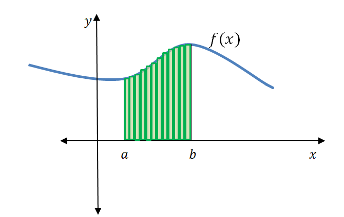
In Unit 1: Introduction to integration, we saw that we could represent the area under a curve using summation notation [latex]\scriptsize \text{A}=\underset{{n\to \infty }}{\mathop{{\lim }}}\,\sum\limits_{{i=1}}^{n}{{f({{x}_{i}})\Delta x}}[/latex]. A sum of this form is called a Riemann sum, named after the 19th-century mathematician Bernhard Riemann, who developed the idea.
Did you know?
Riemann sums are the formal application of the method of exhaustion. You have seen the area under a curve defined in terms of Riemann sums. You can click on this link for a graphical illustration of the definition of Riemann sums.
We saw in unit 1 that since differentiation and integration are inverses, we can easily find the area under a curve by finding definite integrals.
Take note!
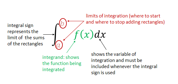 This is called the definite integral and represents the area under a curve, over a given interval and bound by the x-axis.
We have shown that we represent the area under a curve between the x-axis and over a given interval by the definite integral [latex]\scriptsize \int_{a}^{b}{{f(x)dx}}[/latex]. Will the answer to the definite integral be a value or a function?
The answer to the definite integral will be a numerical value because it is giving us the value of the area of a curve between the lower and upper limits of an interval.
[latex]\scriptsize \int_{a}^{b}{{f(x)dx}}=F(b)-F(a)[/latex]
[latex]\scriptsize \int_{a}^{b}{{f(x)dx}}[/latex] tells us that we need to integrate the function [latex]\scriptsize f(x)[/latex] with respect to [latex]\scriptsize x[/latex] over the interval[latex]\scriptsize a[/latex] to [latex]\scriptsize b[/latex].
[latex]\scriptsize F(b)-F(a)[/latex] means we need to find the value of the antiderivative at the upper limit [latex]\scriptsize b[/latex] and subtract from that the value of the antiderivative at the lower limit [latex]\scriptsize a[/latex]. The limits of integration are the x-values or the independent values.
We often use the notation [latex]\scriptsize \left. {F(x)} \right|_{a}^{b}[/latex] to denote the expression [latex]\scriptsize F(b)-F(a)[/latex]. We use the vertical bar and associated limits [latex]\scriptsize \displaystyle a[/latex] and [latex]\scriptsize \displaystyle b[/latex] to indicate that we should evaluate the function [latex]\scriptsize F(x)[/latex] at the upper limit and subtract the value of the function [latex]\scriptsize F(x)[/latex]at the lower limit.
Activity 2.1: Discover the definite integral for different limits of integration
Time required: 15 minutes
What you need:
- a pen and paper
- an internet connection
What to do:
Find [latex]\scriptsize \int_{a}^{b}{{({{x}^{3}}-2{{x}^{2}}-4x+10)dx}}[/latex] for different values of [latex]\scriptsize a[/latex] and [latex]\scriptsize b[/latex].
Step 1: Click on this link to go to the activity.
The following screen should appear.
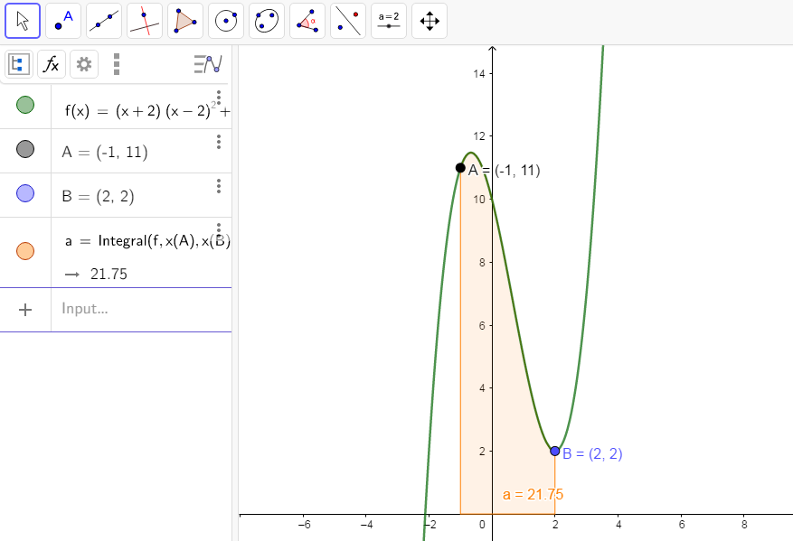
Step 2: From the graph drawn in Geogebra, what is the value of [latex]\scriptsize \int_{a}^{b}{{({{x}^{3}}-2{{x}^{2}}-4x+10)dx}}[/latex] between [latex]\scriptsize \text{A}(-1;11)[/latex] and [latex]\scriptsize \text{B}(2;2)[/latex]? (Hint: This is the value shown as ‘Area a’ on the graph.)
Step 3: Calculate [latex]\scriptsize \int_{{-1}}^{2}{{({{x}^{3}}-2{{x}^{2}}-4x+10)dx}}[/latex]. Show all working. What have you calculated?
Step 4: Using the graph, drag and move point A to [latex]\scriptsize (0;10)[/latex] and drag and move B to [latex]\scriptsize (1;5)[/latex]. You can achieve the same result by just entering the coordinates of A and B on the left of the Geogebra screen as shown here:

What are the limits of integration now?
Step 5: From the graph, read off the integral at the new limits of integration. What does this tell you?
Step 6: Calculate [latex]\scriptsize \int_{0}^{1}{{({{x}^{3}}-2{{x}^{2}}-4x+10)dx}}[/latex]. Show all working. Compare this to your answer from the graph. What do you notice?
What did you find?
- From the graph you can read off the value of [latex]\scriptsize \int_{a}^{b}{{({{x}^{3}}-2{{x}^{2}}-4x+10)dx}}[/latex], where [latex]\scriptsize a=-1[/latex] and [latex]\scriptsize b=2[/latex]. We see that the area between [latex]\scriptsize \text{A}(-1;11)[/latex] and [latex]\scriptsize \text{B}(2;2)[/latex] is [latex]\scriptsize 21.75[/latex].
- Using the rules for integration we can calculate [latex]\scriptsize \int_{{-1}}^{2}{{({{x}^{3}}-2{{x}^{2}}-4x+10)dx}}[/latex] as follows: [latex]\scriptsize \begin{align*}\int_{{-1}}^{2}{{({{x}^{3}}-2{{x}^{2}}-4x+10)dx}}&=\left. {\displaystyle \frac{{{{x}^{4}}}}{4}-\displaystyle \frac{{2{{x}^{3}}}}{3}-\displaystyle \frac{{4{{x}^{2}}}}{2}+10x} \right|_{{-1}}^{2}\\&=\left[ {\displaystyle \frac{{{{2}^{4}}}}{4}-\displaystyle \frac{{2{{{(2)}}^{3}}}}{3}-2{{{(2)}}^{2}}+10(2)} \right]-\left[ {\displaystyle \frac{{{{{(-1)}}^{4}}}}{4}-\displaystyle \frac{{2{{{(-1)}}^{3}}}}{3}-2{{{(-1)}}^{2}}+10(-1)} \right]\\&=\displaystyle \frac{{32}}{3}-(-\displaystyle \frac{{133}}{{12}})\\&=\displaystyle \frac{{87}}{4}\\&=21.75\end{align*}[/latex]
.
You have calculated that the area under the curve between the x-axis and points [latex]\scriptsize \text{A}(-1;11)[/latex]and [latex]\scriptsize \text{B}(2;2)[/latex] is [latex]\scriptsize 21.75[/latex]. This is the same as the answer from the graph. - The limits of integration are the x-values of the co-ordinates of A and B. Therefore, [latex]\scriptsize a=0[/latex] and [latex]\scriptsize b=1[/latex] are the limits of integration.
- From the graph we read that the area is [latex]\scriptsize 7.58[/latex]. This means that the area under the curve and above the x-axis between [latex]\scriptsize (0;10)[/latex] and [latex]\scriptsize (1;5)[/latex] is [latex]\scriptsize 7.58[/latex].
- Use the rules of integration to integrate and then evaluate.
[latex]\scriptsize \displaystyle \begin{align*}\int_{0}^{1}{{({{x}^{3}}-2{{x}^{2}}-4x+10)dx}}&=\left. {\displaystyle \frac{{{{x}^{4}}}}{4}-\displaystyle \frac{{2{{x}^{3}}}}{3}-\displaystyle \frac{{4{{x}^{2}}}}{2}+10x} \right|_{0}^{1}\\&=\left[ {\displaystyle \frac{{{{1}^{4}}}}{4}-\displaystyle \frac{{2{{{(1)}}^{3}}}}{3}-2{{{(1)}}^{2}}+10(1)} \right]-\left[ 0 \right]\\&=\displaystyle \frac{{91}}{{12}}\\&\approx 7.58\end{align*}[/latex]
The answer we calculated is the same as the one shown on the graph as we are also calculating the integral between [latex]\scriptsize (0;10)[/latex] and [latex]\scriptsize (1;5)[/latex]. So we have confirmed that area under the curve and above the x-axis between [latex]\scriptsize (0;10)[/latex] and [latex]\scriptsize (1;5)[/latex] is[latex]\scriptsize 7.58[/latex].
You may recall from unit 1 that we promised to show that [latex]\scriptsize \int_{0}^{1}{{{{x}^{2}}dx}}=\displaystyle \frac{1}{3}[/latex]. This is the same as showing that the area under the curve [latex]\scriptsize f(x)={{x}^{2}}[/latex] between the points [latex]\scriptsize (0;0)[/latex] and [latex]\scriptsize (1,1)[/latex] is equal to exactly [latex]\scriptsize \displaystyle \frac{1}{3}[/latex].
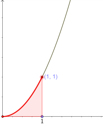
Using [latex]\scriptsize \int_{a}^{b}{{f(x)dx}}=F(b)-F(a)[/latex], we can evaluate the definite integral of [latex]\scriptsize f(x)={{x}^{2}}[/latex] between [latex]\scriptsize [0,1][/latex].
We rewrite this as [latex]\scriptsize \int_{0}^{1}{{{{x}^{2}}dx}}[/latex]. Notice that the upper limit is one and the lower limit is zero and we have replaced [latex]\scriptsize f(x)[/latex] with the function [latex]\scriptsize {{x}^{2}}[/latex]. [latex]\scriptsize \int_{0}^{1}{{{{x}^{2}}dx}}=F(1)-F(0)[/latex] but first we must integrate [latex]\scriptsize f(x)={{x}^{2}}[/latex] using the power rule for integration. You will get that the antiderivative of [latex]\scriptsize {{x}^{2}}[/latex] is [latex]\scriptsize \displaystyle \frac{{{{x}^{3}}}}{3}[/latex].
[latex]\scriptsize \int_{0}^{1}{{{{x}^{2}}dx}}=\left. {\displaystyle \frac{{{{x}^{3}}}}{3}} \right|_{0}^{1}[/latex] Recall that the vertical line with the upper and lower limits means the evaluation of the antiderivative at one, [latex]\scriptsize F(1)[/latex], minus the antiderivative at zero [latex]\scriptsize F(0)[/latex].
By substituting: [latex]\scriptsize F(1)=\displaystyle \frac{{{{1}^{3}}}}{3}=\displaystyle \frac{1}{3}[/latex] and [latex]\scriptsize F(0)=\displaystyle \frac{{{{0}^{3}}}}{3}=0[/latex]
[latex]\scriptsize \therefore \left. {\displaystyle \frac{{{{x}^{3}}}}{3}} \right|_{0}^{1}=\displaystyle \frac{1}{3}-0=\displaystyle \frac{1}{3}[/latex]
In the previous unit we saw that this was the area under the curve [latex]\scriptsize f(x)={{x}^{2}}[/latex] between [latex]\scriptsize [0,1][/latex] using the tiny rectangles, as the number of rectangles increased to infinity. So, we can see that evaluating the definite integral gives exactly the same answer as using the summation of tiny rectangles as [latex]\scriptsize n\to \infty[/latex]. It was this idea that the founders of calculus used to show why differentiation and integration are inverse processes. The fundamental theorem of calculus brings together the two big concepts of integrals and derivatives. Its very name indicates how central this theorem is to the entire development of calculus.
The fundamental theorem of calculus and definite integrals:
If [latex]\scriptsize \displaystyle f[/latex] is continuous over the interval [latex]\scriptsize [a;b][/latex] and [latex]\scriptsize F(x)[/latex] is any antiderivative of[latex]\scriptsize f(x)[/latex], then[latex]\scriptsize \int_{a}^{b}{{f(x)dx}}=\left. {F(x)} \right|_{a}^{b}=F(b)-F(a)[/latex]
The theorem states that if we can find an antiderivative for the integrand, then we can evaluate the definite integral by evaluating the antiderivative at the endpoints of the interval and subtracting.
Did you know?
The fundamental theorem of calculus is made up of two parts. While we have covered both parts of the theorem, this video “Fundamental theorem of calculus (Part 2)” explains both versions of the fundamental theorem of calculus in more detail.
Let us now look at an example.
Example 2.4
- Evaluate [latex]\scriptsize \int\limits_{1}^{4}{{\sqrt{t}(1+t)dt}}[/latex].
- Find the definite integral of [latex]\scriptsize f(x)={{x}^{2}}-3x[/latex] over the interval [latex]\scriptsize [1;5][/latex].
Solutions
- Rewrite the function and simplify using exponent rules.
[latex]\scriptsize \int\limits_{1}^{4}{{\sqrt{t}(1+t)dt}}=\int\limits_{1}^{4}{{{{t}^{{\displaystyle \frac{1}{2}}}}(1+t)dt}}[/latex]
[latex]\scriptsize \int\limits_{1}^{4}{{{{t}^{{\displaystyle \frac{1}{2}}}}(1+t)dt}}=\int\limits_{1}^{4}{{{{t}^{{\displaystyle \frac{1}{2}}}}+{{t}^{{\displaystyle \frac{3}{2}}}}dt}}[/latex] Apply the power rule of integration
[latex]\scriptsize \displaystyle \begin{align*}\int\limits_{1}^{4}{{{{t}^{{\displaystyle \frac{1}{2}}}}+{{t}^{{\displaystyle \frac{3}{2}}}}dt}}&=\left. {\displaystyle \frac{{{{t}^{{\displaystyle \frac{3}{2}}}}}}{{\tfrac{3}{2}}}+\displaystyle \frac{{{{t}^{{\displaystyle \frac{5}{2}}}}}}{{\tfrac{5}{2}}}} \right|_{1}^{4}\\&=\left. {\left( {\displaystyle \frac{2}{3}{{t}^{{\displaystyle \frac{3}{2}}}}+\displaystyle \frac{2}{5}{{t}^{{\displaystyle \frac{5}{2}}}}} \right)} \right|_{1}^{4}\end{align*}[/latex] Use the vertical line with the limits of integration
[latex]\scriptsize \displaystyle \begin{align*}&=\left[ {\displaystyle \frac{2}{3}{{{(4)}}^{{\displaystyle \frac{3}{2}}}}+\displaystyle \frac{2}{5}{{{(4)}}^{{\displaystyle \frac{5}{2}}}}} \right]-\left[ {\displaystyle \frac{2}{3}{{{(1)}}^{{\displaystyle \frac{3}{2}}}}+\displaystyle \frac{2}{5}{{{(1)}}^{{\displaystyle \frac{5}{2}}}}} \right]\\&=\displaystyle \frac{{272}}{{15}}-\displaystyle \frac{{16}}{{15}}\\&=\displaystyle \frac{{256}}{{15}}\end{align*}[/latex] - Rewrite the question in integral notation.
[latex]\scriptsize \int\limits_{1}^{5}{{({{x}^{2}}-3x)}}dx[/latex]
[latex]\scriptsize \begin{align*}\int\limits_{1}^{5}{{({{x}^{2}}-3x)}}dx&=\left. {\displaystyle \frac{{{{x}^{3}}}}{3}-\displaystyle \frac{{3{{x}^{2}}}}{2}} \right|_{1}^{5}\\&=\left[ {\displaystyle \frac{{{{{(5)}}^{3}}}}{3}-\displaystyle \frac{{3{{{(5)}}^{2}}}}{2}} \right]-\left[ {\displaystyle \frac{{{{{(1)}}^{3}}}}{3}-\displaystyle \frac{{3{{{(1)}}^{2}}}}{2}} \right]\\&=\displaystyle \frac{{25}}{6}-(-\displaystyle \frac{7}{6})\\&=\displaystyle \frac{{16}}{3}\end{align*}[/latex]
Exercise 2.3
Evaluate the following definite integrals:
- [latex]\scriptsize \int_{0}^{4}{{(3-x)}}dx[/latex]
- [latex]\scriptsize \displaystyle \int_{{-2}}^{2}{{({{t}^{2}}-4)dt}}[/latex]
- [latex]\scriptsize \int_{0}^{{2\pi }}{{3\cos 2\theta d\theta }}[/latex]
- [latex]\scriptsize \int_{0}^{{\tfrac{\pi }{4}}}{{2{{{\sec }}^{2}}xdx}}[/latex]
- [latex]\scriptsize \int_{1}^{4}{{\left( {\displaystyle \frac{{1+{{x}^{2}}}}{{\sqrt{x}}}} \right)dx}}[/latex]
The full solutions are at the end of the unit.
Summary
In this unit you have learnt the following:
- How to use and apply the integral rules.
- How to find; [latex]\scriptsize \displaystyle \int{{\displaystyle \frac{k}{x}}}dx,\int{{{{e}^{{kx}}}dx,\int{{a\sin kxdx}}}},\int{{a\cos kxdx}},\int{{a{{{\sec }}^{2}}kxdx}}[/latex].
- The fundamental theorem of calculus.
- How to evaluate the definite integral.
Unit 2: Assessment
Suggested time to complete: 35 minutes
- Determine the following integrals (leave your answer with positive exponents and in surd form, where applicable):
- [latex]\scriptsize \int{{(2x-3)(1-2x)dx}}[/latex]
- [latex]\scriptsize \int{{\left( {\displaystyle \frac{{4-4x+{{x}^{2}}}}{{x-2}}} \right)}}dx[/latex]
- [latex]\scriptsize \int{{\left( {{{e}^{{3x}}}+\displaystyle \frac{1}{{{{{\cos }}^{2}}x}}+\displaystyle \frac{{\tan x}}{{\cos x}}} \right)}}dx[/latex]
- [latex]\scriptsize \int{{\left( {2\cos 3x+\displaystyle \frac{{{{e}^{{4x}}}}}{4}+\displaystyle \frac{2}{x}} \right)dx}}[/latex]
- [latex]\scriptsize \int{{\left( {3{{{\sec }}^{2}}2x+2{{e}^{{3x}}}+\displaystyle \frac{1}{x}} \right)dx}}[/latex]
- Evaluate the following:
- [latex]\scriptsize \int_{1}^{3}{{\left( {\displaystyle \frac{{x+1}}{x}} \right)}}dx[/latex]
- [latex]\scriptsize \int_{0}^{\pi }{{\cos 2xdx}}[/latex]
- [latex]\scriptsize \int_{1}^{2}{{\left( {\displaystyle \frac{{{{x}^{4}}+{{x}^{2}}}}{{{{x}^{3}}}}} \right)dx}}[/latex]
The full solutions are at the end of the unit.
Unit 2: Solutions
Exercise 2.1
- .
[latex]\scriptsize \begin{align*}\int{{(2{{x}^{3}}+{{x}^{2}}-2x)dx}}&=2\int{{{{x}^{3}}dx+\int{{{{x}^{2}}dx-2\int{{xdx}}}}}}\\&=2\cdot \displaystyle \frac{{{{x}^{{3+1}}}}}{4}+\displaystyle \frac{{{{x}^{{2+1}}}}}{3}-2\cdot \displaystyle \frac{{{{x}^{{1+1}}}}}{2}+c\\&=\displaystyle \frac{{{{x}^{4}}}}{2}+\displaystyle \frac{{{{x}^{3}}}}{3}-{{x}^{2}}+c\end{align*}[/latex] - .
[latex]\scriptsize \displaystyle \begin{align*}\int{{y(\displaystyle \frac{1}{y}+{{y}^{2}})dy}}&=\int{{(1+{{y}^{3}})dy}}\\&=\int{{1dy+\int{{{{y}^{3}}dy}}}}\\&={{y}^{{0+1}}}+\displaystyle \frac{{{{y}^{{3+1}}}}}{4}+c\\&=y+\displaystyle \frac{{{{y}^{4}}}}{4}+c\end{align*}[/latex] - .
[latex]\scriptsize \displaystyle \begin{align*}\int{{(\sqrt{x}+}}\sqrt{{3x}})dx&=\int{{\sqrt{x}dx+\int{{\sqrt{{3x}}}}}}\\&=\int{{{{x}^{{\displaystyle \frac{1}{2}}}}dx+}}\sqrt{3}\int{{{{x}^{{\displaystyle \frac{1}{2}}}}}}dx\\&=\displaystyle \frac{{{{x}^{{\displaystyle \frac{1}{2}+1}}}}}{{\tfrac{3}{2}}}+\sqrt{3}\cdot \displaystyle \frac{{{{x}^{{\displaystyle \frac{1}{2}+1}}}}}{{\tfrac{3}{2}}}+c\\&=\displaystyle \frac{2}{3}{{x}^{{\displaystyle \frac{3}{2}}}}+\displaystyle \frac{{2\sqrt{3}}}{3}{{x}^{{\displaystyle \frac{3}{2}}}}+c\\&=\displaystyle \frac{{2+2\sqrt{3}}}{3}{{x}^{{\displaystyle \frac{3}{2}}}}+c\end{align*}[/latex]
Exercise 2.2
- .
- [latex]\scriptsize \int{{(x+{{e}^{x}})dx=\displaystyle \frac{1}{2}}}{{x}^{2}}+{{e}^{x}}+c[/latex]
[latex]\scriptsize \begin{align*}F(x)&=\displaystyle \frac{1}{2}{{x}^{2}}+{{e}^{x}}+c\\{F}'(x)&=x+{{e}^{x}}\\f(x)&=x+{{e}^{x}}\\\therefore {F}'(x)&=f(x)\end{align*}[/latex]
The statement [latex]\scriptsize \int{{(x+{{e}^{x}})dx=\displaystyle \frac{1}{2}}}{{x}^{2}}+{{e}^{x}}+c[/latex] is correct. - [latex]\scriptsize \int{{x{{e}^{x}}dx=x{{e}^{x}}-{{e}^{x}}+c}}[/latex]
[latex]\scriptsize \begin{align*}F(x)&=x{{e}^{x}}-{{e}^{x}}+c\\{F}'(x)&=1\cdot {{e}^{x}}+x{{e}^{x}}-{{e}^{x}}+0\text{ Use the product rule}\\&=x{{e}^{x}}\\f(x)&=x{{e}^{x}}\\\therefore {F}'(x)&=f(x)\end{align*}[/latex]
The statement [latex]\scriptsize \int{{x{{e}^{x}}dx=x{{e}^{x}}-{{e}^{x}}+c}}[/latex] is correct. - [latex]\scriptsize \int{{x\cos xdx=x\sin x+\cos x+c}}[/latex]
[latex]\scriptsize \displaystyle \begin{align*}F(x)&=x\sin x+\cos x+c\\{F}'(x)&=\sin x+x\cos x-\sin x\\&=x\cos x\\f(x)&=x\cos x\\\therefore {F}'(x)&=f(x)\end{align*}[/latex] Remember: [latex]\scriptsize {{D}_{x}}[x\sin x]=\sin x+x\cos x[/latex] by the product rule
The statement [latex]\scriptsize \int{{x\cos xdx=x\sin x+\cos x+c}}[/latex] is correct.
- [latex]\scriptsize \int{{(x+{{e}^{x}})dx=\displaystyle \frac{1}{2}}}{{x}^{2}}+{{e}^{x}}+c[/latex]
- .
- [latex]\scriptsize \begin{align*}\int{{\tan x\cos xdx}}&=\int{{\displaystyle \frac{{\sin x}}{{\cos x}}\cos xdx}}\text{ Rewrite }\!\!~\!\!\text{ }\tan x\text{ and simplify}\\&=\int{{\sin xdx}}\end{align*}[/latex]
[latex]\scriptsize \int{{\sin xdx=\cos x+c}}[/latex] - .
[latex]\scriptsize \begin{align*}\int{{\displaystyle \frac{1}{{{{x}^{2}}}}+xdx}}&=\int{{\displaystyle \frac{1}{{{{x}^{2}}}}dx+\int{{xdx}}}}\\&=\int{{{{x}^{{-2}}}dx+\int{{xdx}}}}\text{ }\\&=\displaystyle \frac{{{{x}^{{-2+1}}}}}{{-2+1}}+\displaystyle \frac{{{{x}^{{1+1}}}}}{{1+1}}+c\text{ Use the power rule for integration}\\&=-{{x}^{{-1}}}+\displaystyle \frac{1}{2}{{x}^{2}}+c\\&=\displaystyle \frac{{-1}}{x}+\displaystyle \frac{1}{2}{{x}^{2}}+c\text{ Write answer with positive exponent}\end{align*}[/latex] - [latex]\scriptsize f(x)=5{{x}^{4}}+4{{x}^{5}}+2[/latex] Given [latex]\scriptsize f(x)[/latex] so we can rewrite as [latex]\scriptsize \int{{(5{{x}^{4}}+4{{x}^{5}}+2)}}dx[/latex]
[latex]\scriptsize \begin{align*}\int{{(5{{x}^{4}}+4{{x}^{5}}+2)}}dx&=\displaystyle \frac{{5{{x}^{5}}}}{5}+\displaystyle \frac{{4{{x}^{6}}}}{6}+\displaystyle \frac{{2{{x}^{{0+1}}}}}{1}+c\\&={{x}^{5}}+\displaystyle \frac{2}{3}{{x}^{6}}+2x+c\end{align*}[/latex] - .
[latex]\scriptsize \displaystyle \begin{align*}f(x)&=\displaystyle \frac{1}{{{{x}^{2}}}}\\\therefore \int{\displaystyle \frac{1}{{{x}^{2}}}}dx&=\int{x^{-2}dx}\\&=\displaystyle \frac{{{{x}^{{-1}}}}}{{-1}}+c\\&=-\displaystyle \frac{1}{x}+c\end{align*}[/latex] - .
[latex]\scriptsize \begin{align*}\int{{\left( {2{{{\sec }}^{2}}x+\displaystyle \frac{2}{x}} \right)}}dx&=\int{{2{{{\sec }}^{2}}x}}dx+\int{{\displaystyle \frac{2}{x}}}dx\\&=2\tan x+2\text{In}x+c\end{align*}[/latex] - .
[latex]\scriptsize \begin{align*}\int{{(x-\displaystyle \frac{1}{x}}}{{)}^{2}}dx&=\int{{{{x}^{2}}-}}2+\displaystyle \frac{1}{{{{x}^{2}}}}dx\text{ Multiply out integrand first}\\&=\int{{{{x}^{2}}dx-\int{{2dx+\int{{{{x}^{{-2}}}dx}}}}}}\\&=\displaystyle \frac{{{{x}^{3}}}}{3}-2x+\left( {\displaystyle \frac{{{{x}^{{-1}}}}}{{-1}}} \right)+c\\&=\displaystyle \frac{1}{3}{{x}^{3}}-2x-\displaystyle \frac{1}{x}+c\end{align*}[/latex]
- [latex]\scriptsize \begin{align*}\int{{\tan x\cos xdx}}&=\int{{\displaystyle \frac{{\sin x}}{{\cos x}}\cos xdx}}\text{ Rewrite }\!\!~\!\!\text{ }\tan x\text{ and simplify}\\&=\int{{\sin xdx}}\end{align*}[/latex]
Exercise 2.3
- .
[latex]\scriptsize \begin{align*}\int_{0}^{4}{{(3-x)}}dx&=\int_{0}^{4}{3}dx-\int_{0}^{4}{{xdx}}\\&=\left. {3x-\displaystyle \frac{{{{x}^{2}}}}{2}} \right|_{0}^{4}\\&=\left( {3(4)-\displaystyle \frac{{{{{(4)}}^{2}}}}{2}} \right)-\left( {3(0)-\displaystyle \frac{{{{{(0)}}^{2}}}}{2}} \right)\\&=12-8\\&=4\end{align*}[/latex] - .
[latex]\scriptsize \displaystyle \begin{align*}\int_{{-2}}^{2}{{({{t}^{2}}-4)dt}}&=\left. {\displaystyle \frac{{{{t}^{3}}}}{3}-4t} \right|_{{-2}}^{2}\\&=\left( {\displaystyle \frac{{{{{(2)}}^{3}}}}{3}-4(\displaystyle \frac{2}{3})} \right)-\left( {\displaystyle \frac{{{{{(-2)}}^{3}}}}{3}-4(\displaystyle \frac{{-2}}{3})} \right)\\&=0\end{align*}[/latex] - .
[latex]\scriptsize \int_{0}^{{2\pi }}{{3\cos 2\theta d\theta }}[/latex] Use [latex]\scriptsize \displaystyle \frac{d}{{dx}}a\sin kx=ka\cos kx[/latex] to get [latex]\scriptsize \int{{a\cos kxdx=}}\displaystyle \frac{{a\sin kx}}{k}+c[/latex].
[latex]\scriptsize \int_{0}^{{2\pi }}{{3\cos 2\theta d\theta }}=\left. {\displaystyle \frac{{3\sin 2\theta }}{2}} \right|_{0}^{{2\pi }}[/latex] Where [latex]\scriptsize a=3,k=2[/latex]
[latex]\scriptsize \displaystyle \begin{align*}&=\displaystyle \frac{{3\sin 2(2\pi )}}{2}-\displaystyle \frac{{3\sin 2(0)}}{2}\\&=\displaystyle \frac{{3(0)}}{2}-\displaystyle \frac{{3(0)}}{2}\\&=0\end{align*}[/latex] - .
[latex]\scriptsize \displaystyle \begin{align*}\int_{0}^{{\tfrac{\pi }{4}}}{{2{{{\sec }}^{2}}xdx}}&=\left. {2\tan x} \right|_{0}^{{\tfrac{\pi }{4}}}\\&=2\tan (\displaystyle \frac{\pi }{4})-2\tan (0)\\&=2(1)-2(0)\\&=2\end{align*}[/latex] Using [latex]\scriptsize \int{{a{{{\sec }}^{2}}kxdx=\displaystyle \frac{{a\tan kx}}{k}+c}}[/latex] - .
[latex]\scriptsize \int_{1}^{4}{{\left( {\displaystyle \frac{{1+{{x}^{2}}}}{{\sqrt{x}}}} \right)dx}}=\int_{1}^{4}{{\left( {\displaystyle \frac{1}{{{{x}^{{\tfrac{1}{2}}}}}}+\displaystyle \frac{{{{x}^{2}}}}{{{{x}^{{\tfrac{1}{2}}}}}}} \right)dx}}[/latex] Divide through by the denominator
[latex]\scriptsize \begin{align*}&=\int_{1}^{4}{{\left( {{{x}^{{\displaystyle \frac{{-1}}{2}}}}+{{x}^{{\displaystyle \frac{3}{2}}}}} \right)dx}}\\&=\left. {2{{x}^{{\displaystyle \frac{1}{2}}}}+\displaystyle \frac{{2{{x}^{{\displaystyle \frac{5}{2}}}}}}{5}} \right|_{1}^{4}\\&=\left( {2{{{(4)}}^{{\displaystyle \frac{1}{2}}}}+\displaystyle \frac{{2{{{(4)}}^{{\displaystyle \frac{5}{2}}}}}}{5}} \right)-\left( {2{{{(1)}}^{{\displaystyle \frac{1}{2}}}}+\displaystyle \frac{{2{{{(1)}}^{{\displaystyle \frac{5}{2}}}}}}{5}} \right)\\&=\displaystyle \frac{{84}}{5}-\displaystyle \frac{{12}}{5}\\&=\displaystyle \frac{{72}}{5}\end{align*}[/latex]
Unit 3: Assessment
- .
- .
Expand and simplify first.
[latex]\scriptsize \begin{align*}\int{{(2x-3)(1-2x)dx}}&=\int{{\left( {8x-3-4{{x}^{2}}} \right)}}dx\\&=\int{{8xdx-\int{{3dx-\int{{4{{x}^{2}}dx}}}}}}\\&=\displaystyle \frac{{8{{x}^{2}}}}{2}-3x-\displaystyle \frac{{4{{x}^{3}}}}{3}+c\\&=4{{x}^{2}}-3x-\displaystyle \frac{4}{3}{{x}^{3}}+c\end{align*}[/latex] - .
Factorise and cancel first.
[latex]\scriptsize \displaystyle \begin{align*}\int{{\left( {\displaystyle \frac{{4-4x+{{x}^{2}}}}{{x-2}}} \right)}}dx&=\int{{\left( {\displaystyle \frac{{(2-x)(2-x)}}{{-(2-x)}}} \right)}}dx\\&=\int{{\left( {-(2-x)} \right)dx}}\\&=\int{{(x-2}})dx\\&=\displaystyle \frac{{{{x}^{2}}}}{2}-2x+c\end{align*}[/latex] - .
[latex]\scriptsize \displaystyle \begin{align*}\int{{\left( {{{e}^{{3x}}}+\displaystyle \frac{1}{{{{{\cos }}^{2}}x}}+\displaystyle \frac{{\tan x}}{{\cos x}}} \right)}}dx&=\int{{\left( {{{e}^{{3x}}}+\displaystyle \frac{1}{{{{{\cos }}^{2}}x}}+\tan x\cdot \displaystyle \frac{1}{{\cos x}}} \right)}}dx\\&=\int{{\left( {{{e}^{{3x}}}+{{{\sec }}^{2}}x+\sec x\tan x} \right)}}dx\\&=\int{{{{e}^{{3x}}}}}dx+\int{{{{{\sec }}^{2}}xdx+\int{{\sec x\tan xdx}}}}\\&=\displaystyle \frac{{{{e}^{{3x}}}}}{3}+\tan x+\sec x+c\text{ Since }\displaystyle \frac{d}{{dx}}\sec x=\sec x\tan x\end{align*}[/latex] - .
[latex]\scriptsize \begin{align*}\int{{\left( {2\cos 3x+\displaystyle \frac{{{{e}^{{4x}}}}}{4}+\displaystyle \frac{2}{x}} \right)dx}}&=\displaystyle \frac{{2\sin 3x}}{3}+\displaystyle \frac{{{{e}^{{4x}}}}}{{4\cdot 4}}+2\ln x+c\\&=\displaystyle \frac{2}{3}\sin 3x+\displaystyle \frac{{{{e}^{{4x}}}}}{{16}}+2\ln x+c\end{align*}[/latex] - .
[latex]\scriptsize \begin{align*}\int{{\left( {3{{{\sec }}^{2}}2x+2{{e}^{{3x}}}+\displaystyle \frac{1}{x}} \right)dx}}&=\displaystyle \frac{{3\tan 2x}}{2}+\displaystyle \frac{{2{{e}^{{3x}}}}}{3}+\ln x+c\\&=\displaystyle \frac{3}{2}\tan 2x+\displaystyle \frac{2}{3}{{e}^{{3x}}}+\ln x+c\end{align*}[/latex]
- .
- .
- .
[latex]\scriptsize \begin{align*}\int_{1}^{3}{{\left( {\displaystyle \frac{{x+1}}{x}} \right)}}dx&=\int_{1}^{3}{{\left( {\displaystyle \frac{x}{x}+\displaystyle \frac{1}{x}} \right)}}dx\\&=\int_{1}^{3}{{\left( {1+\displaystyle \frac{1}{x}} \right)}}dx\\&=\left. {x+\ln x} \right|_{1}^{3}\\&=\left( {3+\ln 3} \right)-\left( {1+\ln 1} \right)\\&=3+\ln 3-1\\&=2+\ln 3\end{align*}[/latex] - .
[latex]\scriptsize \begin{align*}\int_{0}^{\pi }{{\cos 2xdx}}&=\left. {\displaystyle \frac{{\sin 2x}}{2}} \right|_{0}^{\pi }\\&=(\displaystyle \frac{{\sin 2\pi }}{2})-(\displaystyle \frac{{\sin 2\left( 0 \right)}}{2})\\&=0\end{align*}[/latex] - .
[latex]\scriptsize \begin{align*}\int_{1}^{2}{{\left( {\displaystyle \frac{{{{x}^{4}}+{{x}^{2}}}}{{{{x}^{3}}}}} \right)dx}}&=\int_{1}^{2}{{\left( {\displaystyle \frac{{{{x}^{4}}}}{{{{x}^{3}}}}+\displaystyle \frac{{{{x}^{2}}}}{{{{x}^{3}}}}} \right)dx}}\\&=\int_{1}^{2}{{\left( {x+\displaystyle \frac{1}{x}} \right)dx}}\\&=\left. {\displaystyle \frac{{{{x}^{2}}}}{2}+\ln x} \right|_{1}^{2}\\&=\left( {\displaystyle \frac{{{{2}^{2}}}}{2}+\ln 2} \right)-\left( {\displaystyle \frac{{{{1}^{2}}}}{2}+\ln 1} \right)\\&=2+\ln 2-\displaystyle \frac{1}{2}\\&=\displaystyle \frac{3}{2}+\ln 2\end{align*}[/latex]
- .
Media Attributions
- Taking the derivative of the antiderivative definition © DHET is licensed under a CC BY (Attribution) license
- Integral notation © DHET is licensed under a CC BY (Attribution) license
- Derivate rule to indefinite integral © DHET is licensed under a CC BY (Attribution) license
- Definite integral introduced © DHET is licensed under a CC BY (Attribution) license
- Area under curve narrowest rectangles © Geogebra is licensed under a CC BY-SA (Attribution ShareAlike) license
- Unit 2 activity screenshot 1 © Geogebra is licensed under a CC BY-SA (Attribution ShareAlike) license
- Unit 2 activity screenshot 2 © DHET is licensed under a CC BY (Attribution) license
- Definite integral over an interval of x^2 © Geogebra is licensed under a CC BY-SA (Attribution ShareAlike) license
