Functions and algebra: Use mathematical models to investigate linear programming problems
Unit 1: Solve linear programming problems by optimising a function
Dylan Busa
Unit outcomes
By the end of this unit you will be able to:
- Determine the linear constraints for a given problem.
- Sketch the linear constraints.
- Find the feasible region.
- Use a search line to optimise the constraints.
What you should know
Before you start this unit, make sure you can:
- Simplify algebraic expressions including those with fractions. Refer to level 2 subject outcome 2.2 unit 1 and 3 if you need help with this.
- Solve linear equations. Refer to level 2 subject outcomes 2.3 unit 1 if you need help with this.
- Solve linear inequalities. Refer to level 3 subject outcome 2.3 unit 3 if you need help with this.
- Sketch graphs of linear functions. Refer to level 2 subject outcome 2.1 unit 1 if you need help with this.
- Sketch constraints given as linear inequalities. Refer to level 3 subject outcome 2.4 unit 1 if you need help with this.
- Find the feasible region defined by the given constraints. Refer to level 3 subject outcome 2.4 unit 1 if you need help with this.
- Define an objective function and optimise this objective function. Refer to level 3 subject outcome 2.4 unit 1 if you need help with this.
Introduction
In level 3 subject outcome 2.4 we were introduced to Qhubeka, the bicycle company that makes and donates bicycles to children in rural areas to make things such as getting to and from school easier and quicker.
We saw how, given a set of constraints, we could optimise how many of each of two types of bicycles the company should make in order to achieve the lowest costs. We called these kinds of problems optimisation problems – considering several given constraints that all need to be taken into account to find an optimal solution.
We also saw that an excellent way to solve optimisation problems was using a graphical technique called linear programming. Linear programming involves:
- assigning variables to the unknowns which we would like to optimise (in the Qhubeka example this was the number of each type of bicycle that should be produced to minimise costs)
- determining and expressing the various constraints in terms of these variables (usually as inequalities)
- sketching these constraints on a graph
- determining the feasible region (the set of all the variables that obey or fulfil all the constraints at the same time)
- determining the objective function or search line to optimise the constraints,
- finding the optimal solution.
In level 3, the expressions for the constraints were always given to you. In this unit, you will need to interpret the given information to determine and express these constraints for yourself. Other than that, everything is the same as you learnt in level 3.
Did you know?
Linear programming is just one of many mathematical modelling techniques. A mathematical model is simply a description of a real-world system or problem using mathematical concepts and language that helps to solve problems, make decisions or predict what might happen in the future.
Watch this informative video that describes mathematical modelling in a little more detail,
“What is Math Modeling?”.
Solve optimisation problems graphically using linear programming
The best way to learn how to solve optimisation problems using linear programming is to work through a few examples before trying some questions on your own.
Example 1.1
A group of learners plans to sell hamburgers and chicken burgers at a rugby match. Their butcher has a total of [latex]\scriptsize 300[/latex] hamburger patties and [latex]\scriptsize 400[/latex] chicken burger patties. Each burger needs to be sold in a packet but there are only [latex]\scriptsize 500[/latex] packets available. Based on past events, the group predicts that demand is likely to be such that the number of chicken burgers sold will be at least half the number of hamburgers sold.
- Write the constraint inequalities and draw a graph of the feasible region.
- Looking at the cost of ingredients, the group plans to make a profit of [latex]\scriptsize \text{R}3.00[/latex] on each hamburger and [latex]\scriptsize \text{R}2.00[/latex] on each chicken burger sold. Write an equation which represents the total profit [latex]\scriptsize P[/latex].
- How many of each type of burger should the group plan to sell if they want to maximise their profits?
Solutions
- We need to write down mathematical expressions of the constraints and draw the feasible region.
Step 1: Assign variables
In this problem, there are two types of burgers to be sold and we want to find out how many of each kind should be made and sold. We need to assign a variable to each type of burger. You can assign any variables you like but, because we will be sketching linear functions, it is often simplest to use [latex]\scriptsize x[/latex] and [latex]\scriptsize y[/latex].
.
Let the number of hamburgers be [latex]\scriptsize x[/latex].
Let the number of chicken burgers be [latex]\scriptsize y[/latex].
.
In both cases, the values of [latex]\scriptsize x[/latex] and [latex]\scriptsize y[/latex] are limited to natural numbers. We cannot sell a fraction of a burger. Therefore [latex]\scriptsize \{x|x\in \mathbb{N}\}[/latex] and [latex]\scriptsize \{y|y\in \mathbb{N}\}[/latex].
.
Step 2: Express the constraints
In level 4, you need to interpret the information given to you to express your own mathematical statements of the constraints.
.
We know that the butcher only has [latex]\scriptsize 300[/latex] hamburger patties and [latex]\scriptsize 400[/latex] chicken burger patties. Therefore, our first two constraints are [latex]\scriptsize x\le 300[/latex] and [latex]\scriptsize y\le 400[/latex].
.
We also know that the total number of burgers sold is limited by the number of packets available. Therefore, our next constraint is [latex]\scriptsize x+y\le 500[/latex].
.
Finally, the group makes a prediction that at least half as many chicken burgers as hamburgers will be sold. Therefore, our final constraint is [latex]\scriptsize x\le 2y[/latex] (or [latex]\scriptsize \displaystyle \frac{1}{2}x\le y[/latex]).
.
Step 3: Graph the constraints
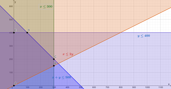
It is time to start graphing our constraints so that we can optimise the objective function. Here they are again.- [latex]\scriptsize x\le 300[/latex]
- [latex]\scriptsize y\le 400[/latex]
- [latex]\scriptsize x+y\le 500[/latex]
- [latex]\scriptsize x\le 2y[/latex]
Here are these constraints graphed. The feasible region is that contained by points [latex]\scriptsize A[/latex], [latex]\scriptsize B[/latex], [latex]\scriptsize C[/latex], [latex]\scriptsize D[/latex] and [latex]\scriptsize E[/latex].
- Now, if a profit of [latex]\scriptsize \text{R}3.00[/latex] is made on each hamburger sold and a profit of [latex]\scriptsize \text{R}2.00[/latex] is made on each chicken burger sold, the profit equation will be [latex]\scriptsize P=3x+2y[/latex]
- To find the maximum profit (the optimum solution), we need to graph our profit function (also called the objective function or the search line) to find what the maximum values for [latex]\scriptsize x[/latex] and [latex]\scriptsize y[/latex] are such that the objective function is still within the feasible region.
.
To sketch the objective function/search line, it is normally best to get the function into standard form.
[latex]\scriptsize \begin{align*}P & =3x+2y\\\therefore 2y & =-3x+P\\\therefore y & =-\displaystyle \frac{3}{2}x+\displaystyle \frac{P}{2}\end{align*}[/latex]
.
In this form, we can see that to maximise the value of [latex]\scriptsize P[/latex] we need to maximise the value of the y-intercept of this straight line. We do not yet know what the value of [latex]\scriptsize P[/latex] is but we do know that the gradient of the graph is [latex]\scriptsize m=-\displaystyle \frac{3}{2}[/latex]. Therefore, we need to sketch any straight line with [latex]\scriptsize m=-\displaystyle \frac{3}{2}[/latex] and then move this line up or down until we get the greatest y-intercept while still having the line pass through at least one point in the feasible region.
.
Here is the objective function/search line graphed such that the profit is maximised. In order to maximise [latex]\scriptsize P[/latex], while still remaining in the feasible region, the objective function must pass through the point [latex]\scriptsize C(300,200)[/latex].
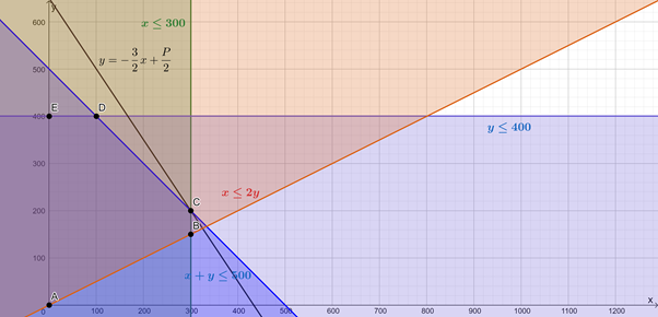
We can either substitute the values for [latex]\scriptsize x[/latex] and [latex]\scriptsize y[/latex] from [latex]\scriptsize C[/latex] into the objective function or we can read off the y-intercept of the function and hence determine the value of [latex]\scriptsize P[/latex].
.
Substituting [latex]\scriptsize C(300,200)[/latex]:
[latex]\scriptsize \begin{align*}P&=3(300)+2(200)\\&=900+400\\&=1\ 300\end{align*}[/latex]
.
Reading off the y-intercept:
y-intercept is [latex]\scriptsize 650[/latex]
[latex]\scriptsize \begin{align*}\therefore \displaystyle \frac{P}{2}&=650\\\therefore P&=1\ 300\end{align*}[/latex]
.
This means that to make a maximum profit, the group must sell [latex]\scriptsize 300[/latex] hamburgers and [latex]\scriptsize 200[/latex] chicken burgers. This will generate a maximum profit of [latex]\scriptsize \text{R}1\ 300.00[/latex].
Note
If you would like to play with an interactive version of the solution to Example 1.1, please visit this link.
Example 1.2
Question adapted from NC(V) Mathematics Level 4 Paper 1 October 2013 question 4.5
A patient is required to take at least [latex]\scriptsize 18[/latex] grams of protein, [latex]\scriptsize 6[/latex] milligrams of vitamin C, and [latex]\scriptsize 5[/latex] milligrams of iron per meal which consists of two types of food, A and B. Type A contains [latex]\scriptsize 9[/latex] grams of protein, [latex]\scriptsize 6[/latex] milligrams of vitamin C and no iron per mass unit. Type B contains [latex]\scriptsize 3[/latex] grams of protein, [latex]\scriptsize 2[/latex] milligrams of vitamin C and [latex]\scriptsize 5[/latex] milligrams of iron per mass unit. The energy value of A is [latex]\scriptsize 800[/latex] kilojoules and that of B is [latex]\scriptsize 400[/latex] kilojoules per mass unit. A patient is not allowed to have more than [latex]\scriptsize 4[/latex] mass units of A and [latex]\scriptsize 5[/latex] mass units of B. There are [latex]\scriptsize x[/latex] mass units of A and [latex]\scriptsize y[/latex] mass units of B on the patient’s plate. The patient cannot eat a fraction of a mass unit of either type of food.
- Write down all the constraints with respect to the above information in terms of [latex]\scriptsize x[/latex] and [latex]\scriptsize y[/latex].
- What is the kilojoule intake per meal?
- Represent the constraints graphically.
- Deduce from the graphs the values of [latex]\scriptsize x[/latex] and [latex]\scriptsize y[/latex] that give the minimum kilojoule intake per meal for the patient.
Solutions
- We are told that the mass units of food type A are [latex]\scriptsize x[/latex] and the mass units of food type B are [latex]\scriptsize y[/latex]. We are also told that the patient can have at most [latex]\scriptsize 4[/latex] mass units of A and [latex]\scriptsize 5[/latex] mass units of B. Therefore, [latex]\scriptsize x\le 4[/latex] and [latex]\scriptsize y\le 5[/latex]. Remember, however, that we cannot have fractions of mass units. Therefore, [latex]\scriptsize x\in \mathbb{N}[/latex] and [latex]\scriptsize y\in \mathbb{N}[/latex].
.
We are also told about the nutrient content of each food and how much of each nutrient the patient needs. The patient needs at least [latex]\scriptsize 18[/latex] grams of protein per meal. Food type A gives [latex]\scriptsize 9[/latex] grams and food type B gives [latex]\scriptsize 3[/latex] grams. Therefore, [latex]\scriptsize 9x+3y\ge 18[/latex].
.
The patient needs at least 6 milligrams of vitamin C per meal. Food type A gives [latex]\scriptsize 6[/latex] milligrams and food type B gives [latex]\scriptsize 2[/latex] milligrams. Therefore, [latex]\scriptsize 6x+2y\ge 6[/latex].
.
Finally, the patient needs at least [latex]\scriptsize 5[/latex] milligrams of iron per meal. Food type A gives [latex]\scriptsize 0[/latex] milligrams and food type B gives [latex]\scriptsize 5[/latex] milligrams. Therefore, [latex]\scriptsize 5y\ge 5[/latex] - Food type A has [latex]\scriptsize 800[/latex] kilojoules and food type B has [latex]\scriptsize 400[/latex] kilojoules. Therefore, the total energy ([latex]\scriptsize \displaystyle E[/latex]) intake is [latex]\scriptsize E=800x+400y[/latex].
- It makes it easier to sketch the constraints if they are all in standard form.
[latex]\scriptsize \begin{align*}9x+3y & \ge 18\\\therefore 3y & \ge -9x+18\\\therefore y & \ge -3x+6\end{align*}[/latex]
[latex]\scriptsize \begin{align*}6x+2y & \ge 6\\\therefore 2y & \ge -6x+6\\\therefore y & \ge -3x+3\end{align*}[/latex]
[latex]\scriptsize \begin{align*}5y & \ge 5\\\therefore y & \ge 1\end{align*}[/latex]
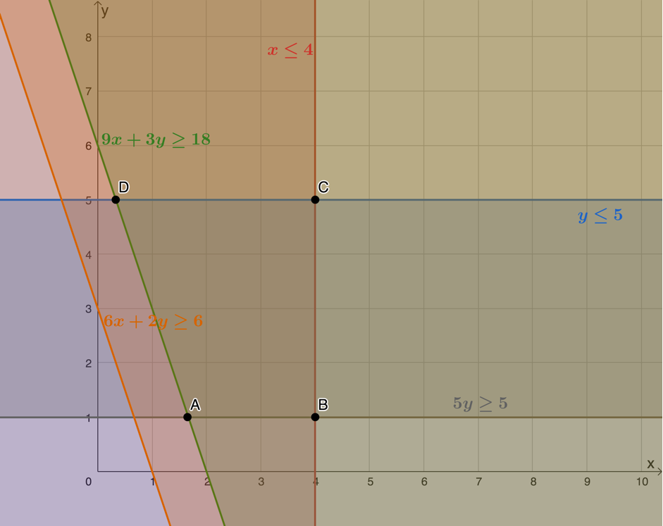
Here are these constraints graphed. The feasible region is that contained by points [latex]\scriptsize A[/latex], [latex]\scriptsize B[/latex], [latex]\scriptsize C[/latex] and [latex]\scriptsize D[/latex].
- We have an equation for the kilojoule intake (the objective function) and we are asked to find the minimum intake. In other words, we need to minimise the function. If we write the objective function in standard form, we will see that the minimum value for [latex]\scriptsize E[/latex] corresponds to the minimum y-intercept that the function or search line can achieve while still passing through the feasible region. Here is the objective function in standard form.
[latex]\scriptsize \begin{align*} E&=800x+400y\\ \therefore 400y&=-800x+E\\ \therefore y&=-2x+\displaystyle \frac{E}{400} \end{align*}[/latex]
Here is a plot of the objective function. We can see that the minimum value is achieved when the function passes through [latex]\scriptsize A[/latex].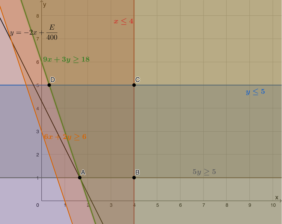 However, we need to remember that [latex]\scriptsize x\in \mathbb{N}[/latex] and [latex]\scriptsize y\in \mathbb{N}[/latex]. Point [latex]\scriptsize A[/latex] represents a value of [latex]\scriptsize x[/latex] that is not an integer, therefore, we need to move the objective function so that it passes through the next available point in the feasible region where both coordinates are integers. This is represented by point [latex]\scriptsize E(2,1)[/latex].
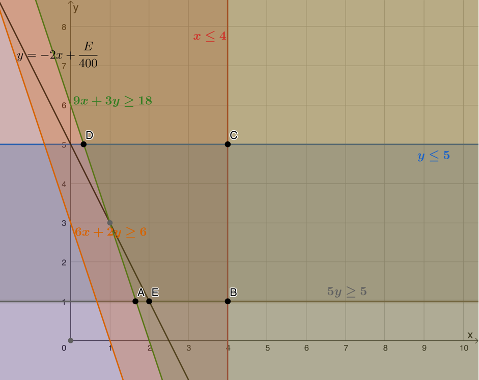
Once again, we can determine what the minimum value of [latex]\scriptsize E[/latex] is by substituting the coordinates of point [latex]\scriptsize E[/latex] into the objective function or by determining the y-intercept and then using the fact that the y-intercept is equal to [latex]\scriptsize \displaystyle \frac{E}{{400}}[/latex].
.
Substituting [latex]\scriptsize E(2,1)[/latex]:
[latex]\scriptsize \begin{align*}E&=800(2)+400(1)\\&=1\ 600+400\\&=2\ 000\end{align*}[/latex]
.
Reading off the y-intercept:
y-intercept is [latex]\scriptsize 5[/latex]
[latex]\scriptsize \begin{align*}\therefore \displaystyle \frac{E}{{400}} & =5\\\therefore E & =2\ 000\end{align*}[/latex]
The minimum kilojoule intake the patient can have is [latex]\scriptsize 2\ 000[/latex] kilojoules and this corresponds to eating [latex]\scriptsize 2[/latex] mass units of food type A and [latex]\scriptsize 1[/latex] mass unit of food type B.
Note
If you would like to play with an interactive version of the solution to example 1.2, please visit this link.
Exercise 1.1
Question 1 adapted from NC(V) Mathematics Level 4 Paper 1 November 2016 question 3
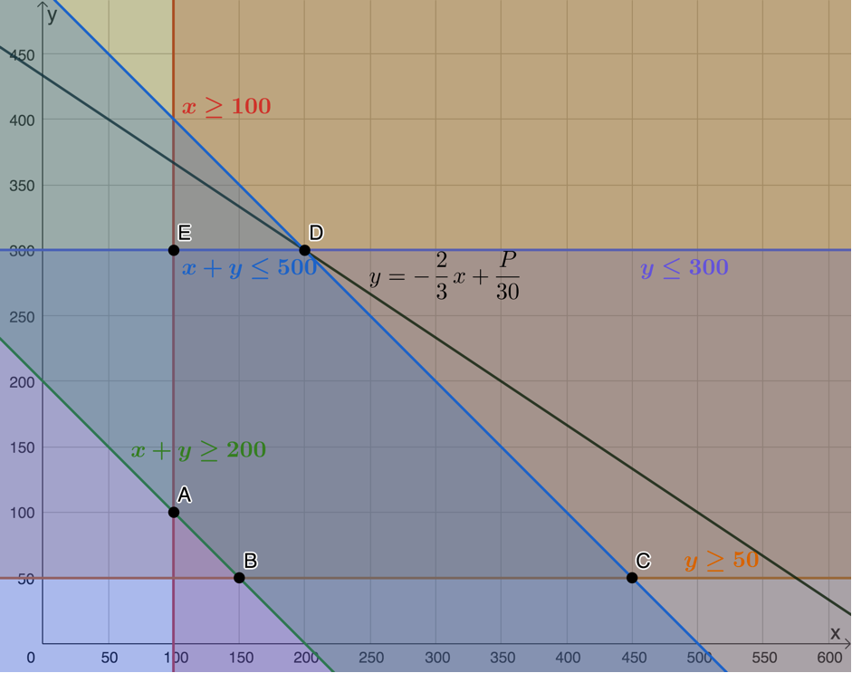
- A small sugar company produces brown sugar and white sugar. In order for the company to be economically viable, it must produce at least [latex]\scriptsize 200[/latex] boxes of sugar daily. The company can produce a maximum of [latex]\scriptsize 500[/latex] boxes of sugar daily. At least [latex]\scriptsize 100[/latex] boxes of brown sugar are to be produced per day. At least [latex]\scriptsize 50[/latex] boxes and at most [latex]\scriptsize 300[/latex] boxes of white sugar must be produced daily.
.
Let [latex]\scriptsize x[/latex] be the number of boxes of brown sugar and [latex]\scriptsize y[/latex] be the number of boxes of white sugar that are produced each day.- Write down all the algebraic inequalities (in terms of [latex]\scriptsize x[/latex] and [latex]\scriptsize y[/latex]) which describe the constraints related to the production of sugar.
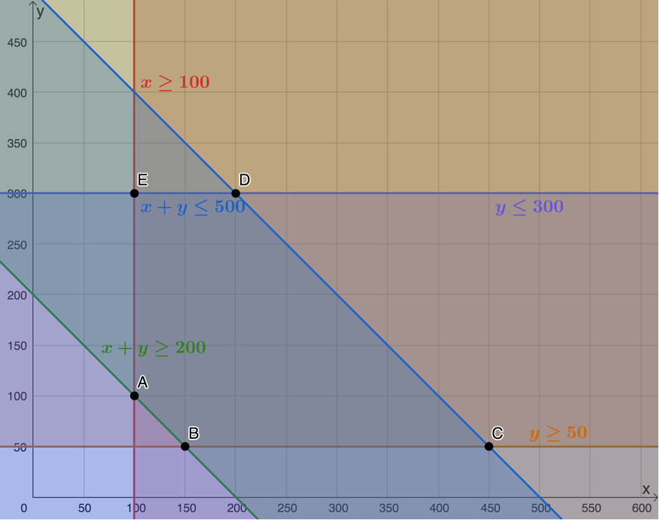
- Represent the inequalities in a. graphically and clearly indicate (shade and label) the feasible region.
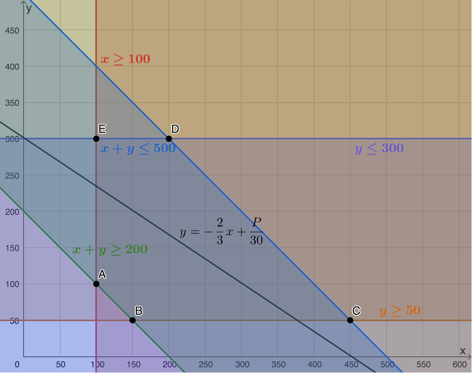
- A profit of [latex]\scriptsize \text{R}20.00[/latex] is made on a box of brown sugar and profit of [latex]\scriptsize \text{R}30.00[/latex] on a box of white sugar. Use this information to draw, on the graph for b., a profit search-line.
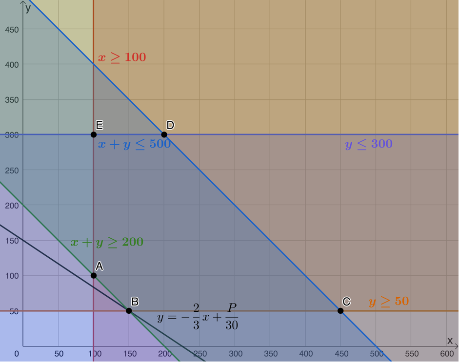
- Use the profit search-line to calculate the minimum and maximum profit the company can make each day.
Question 2 adapted from NC(V) Mathematics Level 4 Paper 1 November 2015 question 5
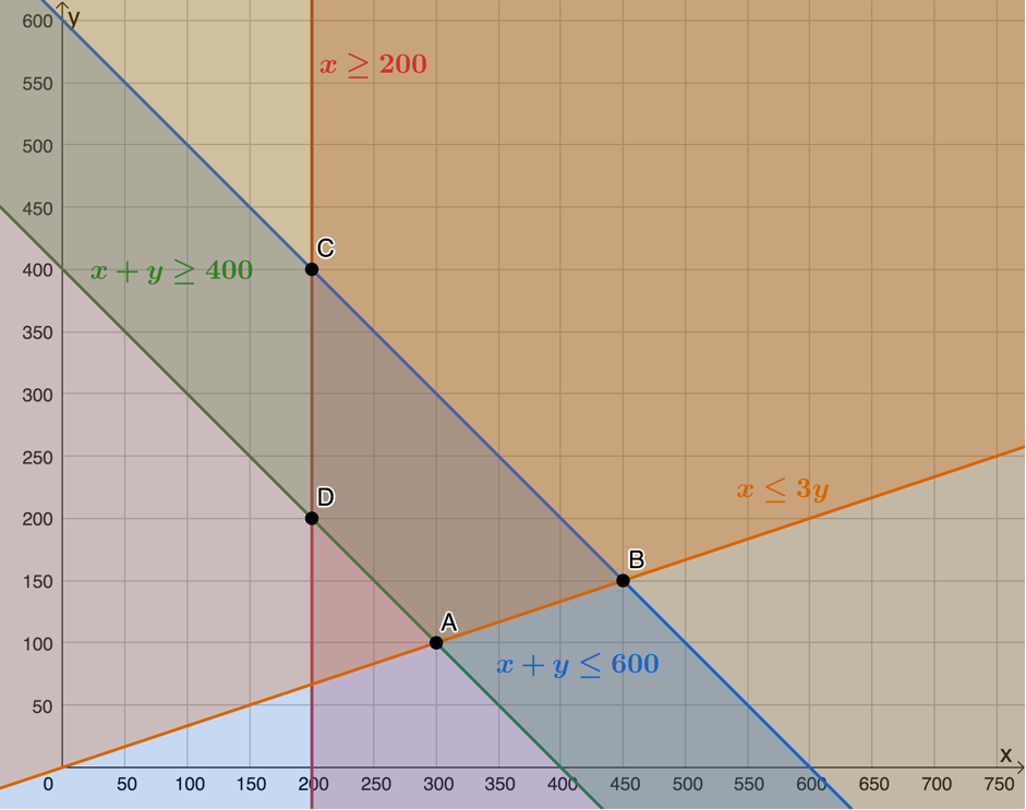
- A transport company uses buses and minibuses to transport a minimum of [latex]\scriptsize 400[/latex] passengers and a maximum of [latex]\scriptsize 600[/latex] passengers each day. At least [latex]\scriptsize 200[/latex] passengers per day must be transported by bus. The number of passengers travelling by bus cannot be more than three times the number of passengers travelling by minibus. Let [latex]\scriptsize x[/latex] represent the number of passengers transported by bus and [latex]\scriptsize y[/latex] be the number of passengers transported by minibus.
- Determine the constraints, in terms of [latex]\scriptsize x[/latex] and [latex]\scriptsize y[/latex], under which the transport company operates.
- Represent the constraints graphically and clearly indicate the feasible region.
- The profit per day per passenger travelling by bus is [latex]\scriptsize \text{R}2.00[/latex] and the profit per day per passenger travelling by minibus is [latex]\scriptsize \text{R}1.60[/latex]. Determine from your graph by means of a search line, the values of [latex]\scriptsize x[/latex] and [latex]\scriptsize y[/latex] that will yield a maximum profit.
- Calculate the maximum possible profit per day.
The full solutions are at the end of the unit.
Summary
In this unit you have learnt the following:
- How to determine and express the constraints for a given problem as linear inequalities.
- How to sketch the constraints on a Cartesian plane.
- How to find and mark the feasible region.
- How to define the objective function (or search line) from given information
- How to use this objective function (or search line) to determine the optimal solution.
Unit 1: Assessment
Suggested time to complete: 15 minutes
Question 1 adapted from NC(V) Mathematics Level 4 Paper 1 November 2012 question 1.3
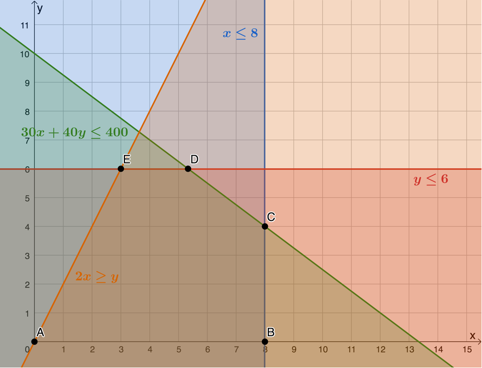
- A carpenter makes two types of tables, A and B.
-
- He has [latex]\scriptsize 400\ {{\text{m}}^{2}}[/latex] of floor space available.
- Each table A requires [latex]\scriptsize 30\ {{\text{m}}^{2}}[/latex] of floor space and each table B requires [latex]\scriptsize 40\ {{\text{m}}^{2}}[/latex] of floor space.
- He does not have enough skilled labourers to make more than [latex]\scriptsize 8[/latex] tables of type A and [latex]\scriptsize 6[/latex] of type B.
- According to public demand he has to make at most two type A tables for each type B table.
.
Let [latex]\scriptsize x[/latex] be the number of tables of type A and [latex]\scriptsize y[/latex] the number of tables of type B.
- Write the constraints with respect to the above information in terms of [latex]\scriptsize x[/latex] and [latex]\scriptsize y[/latex].
- Represent graphically ALL the constraint inequalities and clearly indicate the feasible region.
- If the profit made on each table is the same, determine by means of a search line, how many of each type of table should be made for maximum profit.
-
Question 2 adapted from NC(V) Mathematics Level 4 Paper 1 November 2011 question 1.3
- Jackson’s clothing factory manufactures jackets and jerseys. A maximum of [latex]\scriptsize 60[/latex] jackets and [latex]\scriptsize 40[/latex] jerseys can be manufactured daily while in total not more than [latex]\scriptsize 70[/latex] pieces of clothing can be manufactured per day. It takes [latex]\scriptsize 5[/latex] hours to manufacture a jacket and [latex]\scriptsize 10[/latex] hours to manufacture a jersey, while there are at most [latex]\scriptsize 500[/latex] working hours available per day.
.
Let [latex]\scriptsize x[/latex] represent the number of jackets and [latex]\scriptsize y[/latex] represents the number of jerseys manufactured per day.- Write down the constraints with respect to the above information in terms of [latex]\scriptsize x[/latex] and [latex]\scriptsize y[/latex].
- Represent all the constraint inequalities on the grid and clearly indicate the feasible region.
- If the profit is [latex]\scriptsize \text{R}15[/latex] on a jacket and [latex]\scriptsize \text{R}25[/latex] on a jersey, give the equation that indicates the profit.
- Using the search line method, determine how many jackets and how many jerseys should be manufactured in order to obtain the maximum profit?
- Determine the maximum profit.
Question 3 adapted from NC(V) Mathematics Level 4 Paper 1 October 2014 question 5
- A trucking company wants to purchase a maximum of [latex]\scriptsize 15[/latex] new trucks that will provide at least [latex]\scriptsize 36[/latex] tons of additional shipping capacity. A model A truck holds [latex]\scriptsize 2[/latex] tons and costs [latex]\scriptsize \text{R}150\ 000[/latex]. A model B truck holds [latex]\scriptsize 3[/latex] tons and costs [latex]\scriptsize \text{R}240\ 000[/latex].
.
Let [latex]\scriptsize x[/latex] be the number of model A trucks and let [latex]\scriptsize y[/latex] be the number of model B trucks.- Write down the constraints that represent the above information.
- Represent the system of constraints on the grid indicating the feasible region by means of shading.
- How many trucks of each model should the company purchase in order to provide the additional shipping capacity at minimum cost?
- Calculate the minimum cost.
The full solutions are at the end of the unit.
Unit 1: Solutions
Exercise 1.1
- .
- Number of boxes of brown sugar is [latex]\scriptsize x[/latex], [latex]\scriptsize x\in \mathbb{N}[/latex]
Number of boxes of white sugar is [latex]\scriptsize y[/latex], [latex]\scriptsize y\in \mathbb{N}[/latex]
Minimum number of boxes of sugar: [latex]\scriptsize x+y\ge 200[/latex]
Maximum number of boxes of sugar: [latex]\scriptsize x+y\le 500[/latex]
Minimum number of boxes of brown sugar: [latex]\scriptsize x\ge 100[/latex]
Minimum number of boxes of white sugar: [latex]\scriptsize y\ge 50[/latex]
Maximum number of boxes of white sugar: [latex]\scriptsize y\le 300[/latex] - The feasible region is bound by points [latex]\scriptsize A[/latex], [latex]\scriptsize B[/latex], [latex]\scriptsize C[/latex], [latex]\scriptsize D[/latex], and [latex]\scriptsize E[/latex].
- .
[latex]\scriptsize \begin{align*}P&=20x+30y\\ \therefore 30y&=-20x+P\\ \therefore y&=-\displaystyle \frac{2}{3}x+\displaystyle \frac{P}{30} \end{align*}[/latex]
- Minimum profit occurs when the objective function or search line passes through [latex]\scriptsize B(150,50)[/latex]. Therefore, the minimum profit is:
[latex]\scriptsize \begin{align*}P&=20(150)+30(50)\\&=3\ 000+1\ 500\\&=4\ 500\end{align*}[/latex]
Maximum profit occurs when the objective function or search line passes through [latex]\scriptsize D(200,300)[/latex]. Therefore, maximum profit is:
[latex]\scriptsize \begin{align*}P&=20(200)+30(300)\\&=4\ 000+9\ 000\\&=13\ 000\end{align*}[/latex]
Visit the interactive solution.
.
- Number of boxes of brown sugar is [latex]\scriptsize x[/latex], [latex]\scriptsize x\in \mathbb{N}[/latex]
- .
- Passengers transported by bus is [latex]\scriptsize x[/latex], [latex]\scriptsize x\in \mathbb{N}[/latex]
Passengers transported by minibus is [latex]\scriptsize y[/latex], [latex]\scriptsize y\in \mathbb{N}[/latex]
Minimum number of passengers per day: [latex]\scriptsize x+y\ge 400[/latex]
Maximum number of passengers per day: [latex]\scriptsize x+y\le 600[/latex]
Minimum number of bus passengers: [latex]\scriptsize x\ge 200[/latex]
Bus passengers cannot be more than three times minibus passengers: [latex]\scriptsize x\le 3y[/latex] - Feasible region is bound by points [latex]\scriptsize A[/latex], [latex]\scriptsize B[/latex], [latex]\scriptsize C[/latex] and [latex]\scriptsize D[/latex].
- .
[latex]\scriptsize \begin{align*}P & =2x+1.6y\\\therefore 1.6y & =-2x+P\\\therefore y & =-\displaystyle \frac{2}{{1.6}}x+\displaystyle \frac{P}{{1.6}}\\\therefore y & =-\displaystyle \frac{5}{4}x+\displaystyle \frac{P}{{1.6}}\end{align*}[/latex]
Maximum profit will occur when the objective function or search lines passes through point [latex]\scriptsize B(450,150)[/latex].
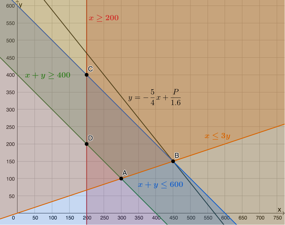
- The maximum profit is:
[latex]\scriptsize \begin{align*}P&=2(450)+1.6(150)\\&=900+240\\&=1\ 140\end{align*}[/latex]
.
Visit the interactive solution.
.
- Passengers transported by bus is [latex]\scriptsize x[/latex], [latex]\scriptsize x\in \mathbb{N}[/latex]
Unit 1: Assessment
- .
- Table type A is [latex]\scriptsize x[/latex], [latex]\scriptsize x\in \mathbb{N}[/latex]
Table type B is [latex]\scriptsize y[/latex], [latex]\scriptsize y\in \mathbb{N}[/latex]
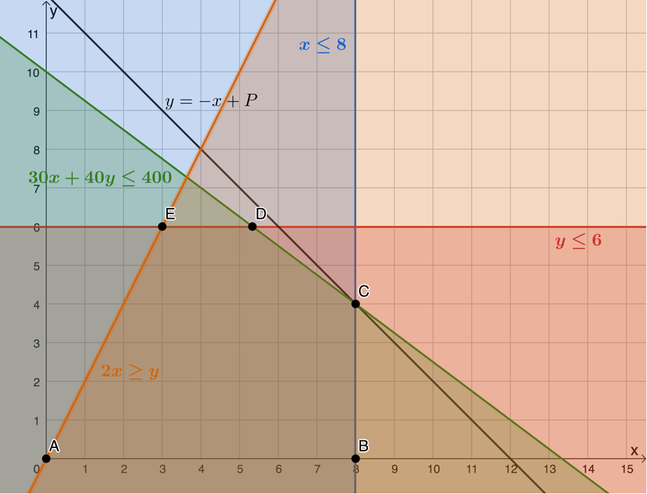
Floor space available: [latex]\scriptsize 30x+40y\le 400[/latex]
Maximum type A tables: [latex]\scriptsize x\le 8[/latex]
Maximum type B tables: [latex]\scriptsize y\le 6[/latex]
At most two type A tables for each type B table: [latex]\scriptsize 2x\ge y[/latex] - Feasible region is bound by points [latex]\scriptsize A[/latex], [latex]\scriptsize B[/latex], [latex]\scriptsize C[/latex], [latex]\scriptsize D[/latex] and [latex]\scriptsize E[/latex].
- .
[latex]\scriptsize \begin{align*}P & =x+y\\\therefore y & =-x+P\end{align*}[/latex]
Maximum profit occurs when the objective function or search line passes through [latex]\scriptsize C(8,4)[/latex]. Therefore, [latex]\scriptsize 8[/latex] units of table A and [latex]\scriptsize 4[/latex] units of table B should be made to maximise profit.
.
Visit the interactive solution.
.
- Table type A is [latex]\scriptsize x[/latex], [latex]\scriptsize x\in \mathbb{N}[/latex]
- .
- Number of jackets is [latex]\scriptsize x[/latex], [latex]\scriptsize x\in \mathbb{N}[/latex]
Number of jerseys is [latex]\scriptsize y[/latex], [latex]\scriptsize y\in \mathbb{N}[/latex]
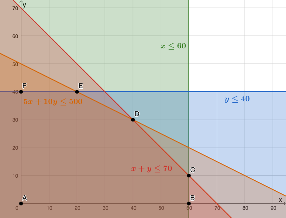
Maximum jackets: [latex]\scriptsize x\le 60[/latex]
Maximum jerseys: [latex]\scriptsize y\le 40[/latex]
Maximum pieces of clothing: [latex]\scriptsize x+y\le 70[/latex]
Working hours available: [latex]\scriptsize 5x+10y\le 500[/latex] - Feasible region is bound by points [latex]\scriptsize A[/latex], [latex]\scriptsize B[/latex], [latex]\scriptsize C[/latex], [latex]\scriptsize D[/latex], [latex]\scriptsize E[/latex] and [latex]\scriptsize F[/latex].
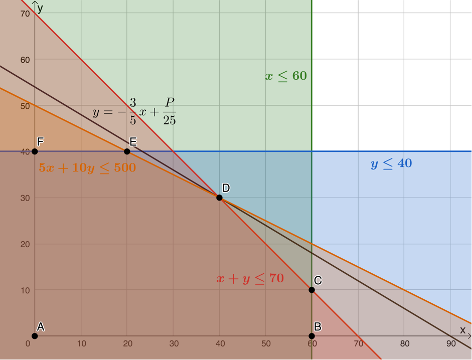
- [latex]\scriptsize P=15x+25y[/latex]
- .
[latex]\scriptsize \begin{align*} P&=15x+25y\\ \therefore 25y&=-15x+P\\ \therefore y&=-\displaystyle \frac{3}{5}x+\displaystyle \frac{P}{25}\end{align*}[/latex]
Profit is at a maximum when the objective function of the search line passes through [latex]\scriptsize D(40,30)[/latex].
- .
[latex]\scriptsize \begin{align*} P&=15(40)+25(30)\\&=600+750\\&=1~350\end{align*}[/latex]
The maximum profit is [latex]\scriptsize \text{R}1\ 350.00[/latex].
.
Visit the interactive solution.
.
- Number of jackets is [latex]\scriptsize x[/latex], [latex]\scriptsize x\in \mathbb{N}[/latex]
- .
- Number of model A trucks is [latex]\scriptsize x[/latex], [latex]\scriptsize x\in \mathbb{N}[/latex]
Number of model B trucks is [latex]\scriptsize y[/latex], [latex]\scriptsize y\in \mathbb{N}[/latex]
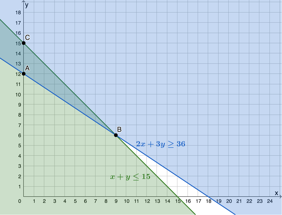
Maximum number of trucks: [latex]\scriptsize x+y\le 15[/latex]
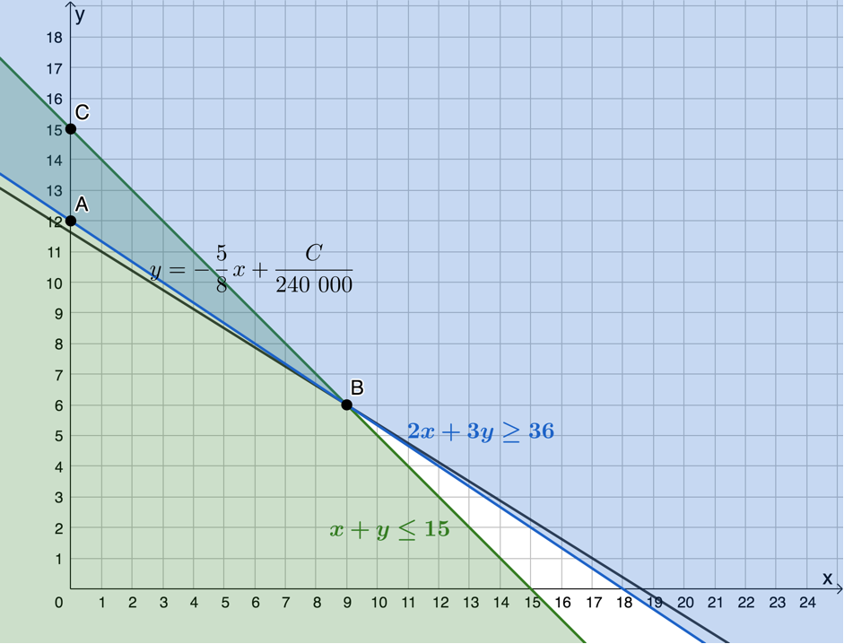
Minimum shipping capacity: [latex]\scriptsize 2x+3y\ge 36[/latex] - Feasible region is bound by points [latex]\scriptsize A[/latex], [latex]\scriptsize B[/latex] and [latex]\scriptsize C[/latex].
- The total cost of the trucks will be [latex]\scriptsize C=150\ 000x+240\ 000y[/latex]. To plot and minimise this objective function we get it into standard form.
[latex]\scriptsize \displaystyle \begin{align*}C & =150\ 000x+240\ 000y\\\therefore 240\ 000y & =-150\ 000x+C\\\therefore y & =-\displaystyle \frac{5}{8}x+\displaystyle \frac{C}{{240\ 000}}\end{align*}[/latex]
Cost is at a minimum when the objective function passes through [latex]\scriptsize B(9,6)[/latex]. [latex]\scriptsize 9[/latex] model A trucks and [latex]\scriptsize 6[/latex] model B trucks should be purchased to minimise the cost.
- .
[latex]\scriptsize \begin{align*}C&=150~000(9)+240~000(6)\\&=1~350~000+1~440~000\\&=2~790~000\end{align*}[/latex]
The minimum cost will be [latex]\scriptsize \text{R}2\ 790\ 000[/latex].
.
Visit the interactive solution.
.
- Number of model A trucks is [latex]\scriptsize x[/latex], [latex]\scriptsize x\in \mathbb{N}[/latex]
Media Attributions
- example1.1 A1 © Geogebra is licensed under a CC BY-SA (Attribution ShareAlike) license
- example1.1 A3 © Geogebra is licensed under a CC BY-SA (Attribution ShareAlike) license
- example1.2 A3 © Geogebra is licensed under a CC BY-SA (Attribution ShareAlike) license
- example1.2 A4.1 © Geogebra is licensed under a CC BY-SA (Attribution ShareAlike) license
- example1.2 A4.2 © Geogebra is licensed under a CC BY-SA (Attribution ShareAlike) license
- exercise1.1 A1b © Geogebra is licensed under a CC BY-SA (Attribution ShareAlike) license
- exercise1.1 A1c © Geogebra is licensed under a CC BY-SA (Attribution ShareAlike) license
- exercise1.1 A1d1 © Geogebra is licensed under a CC BY-SA (Attribution ShareAlike) license
- exercise1.1 A1d2 © Geogebra is licensed under a CC BY-SA (Attribution ShareAlike) license
- exercise1.1 A2b © Geogebra is licensed under a CC BY-SA (Attribution ShareAlike) license
- exercise1.1 A2c © Geogebra is licensed under a CC BY-SA (Attribution ShareAlike) license
- assessment A1b © Geogebra is licensed under a CC BY-SA (Attribution ShareAlike) license
- assessment A1c © Geogebra is licensed under a CC BY-SA (Attribution ShareAlike) license
- assessment A2b © Geogebra is licensed under a CC BY-SA (Attribution ShareAlike) license
- assessment A2d © Geogebra is licensed under a CC BY-SA (Attribution ShareAlike) license
- assessment A3b © Geogebra is licensed under a CC BY-SA (Attribution ShareAlike) license
- assessment A3c © Geogebra is licensed under a CC BY-SA (Attribution ShareAlike) license
